
Microeconomics is the study of individuals and business decisions, whereas macroeconomics considers the decisions of nations and governments. Though these two branches of economics appear to be varied, they are interdependent and complement one another. Many overlapping issues exist between the two fields. Microeconomics and macroeconomics are two branches of economics that analyze different aspects of economic behavior and outcomes at different levels of aggregation. While microeconomics focuses on individual agents and markets, macroeconomics examines the economy as a whole. Understanding the principles and concepts of both branches is essential for comprehending the functioning of economies and informing policy decisions.
Microeconomics Meaning
Microeconomics is the branch of economics that focuses on the behavior of individual agents and specific markets within the economy. It examines how individual consumers, firms, and households make decisions regarding the allocation of resources and how their interactions in markets determine prices, quantities, and resource allocation. Key topics in microeconomics include supply and demand, consumer behavior, production and costs, market structures (such as perfect competition and monopoly), and the allocation of resources.
Nature of Microeconomics
The terms „microeconomics‟ and „macroeconomics‟ have been coined by a Norwegian economist Ragnar Frisch in 1933. The word micro is derived from a Greek word mikros which means small. When economic problems or economic issues are studied considering small economic units like an individual consumer or an individual producer, we are referring to microeconomics. The basic economic problem is the problem of choice related to allocation of scarce resources to alternative uses at an individual level ( both consumer & producer). As Gardner Ackley says, “Microeconomics deals with the division of total output among industries, products and firms and the allocation of resources among competing groups. It considers problems of income distribution. Its interest is in relative prices of particular goods and services.” According to Maurice Dobb, Microeconomics is, in fact, a microscopic study of the economy. It is like looking at the economy through a microscope to find out the working of markets for individual commodities and the behavior of individual consumers and producers.
Scope of Microeconomics
The scope or the subject matter of microeconomics is concerned with:
- Product Pricing: The price of an individual commodity is determined by the market forces of demand and supply. Demand for goods and services and consumer‟s choice on the allocation of his income to different uses are the issues studied in the theory of consumer behavior or theory of demand and the problems faced by a producer in deciding the product and combination of inputs used comes under the theory of producer behavior or theory of supply.
- Factor Pricing Theory: Microeconomics helps in determining the factor prices for land, labor, capital and entrepreneurship in the form of rent ,wages, interest and profit respectively. These are the factors which contribute to the production process.
- Theory of Economic Welfare: The welfare component in microeconomics is concerned with solving the problems in attaining economic efficiency to maximize public welfare. It attempts to gain efficiency in production, consumption/distribution to attain overall efficiency and provides answers for „What to produce?‟, „When to produce?‟, „How to produce?‟, and „For whom to produce?‟.
Importance of Microeconomics
- Individual Behaviour Analysis: Microeconomics helps in studying the behaviour of individual consumer or producer in different situations where individual has freedom to take his own economic decisions.
- Resource Allocation: We know that resources are limited in nature as compared to their demand and for that we have to use them judiciously. Microeconomics helps in proper allocation and utilization of these scarce resources to produce various types of goods and services.
- Tools for Economic Policies: Microeconomics through price or market mechanism helps the state in formulating correct price policies and their evaluation in proper perspective.
- Economic Policy: Microeconomics helps in the formulation of economic plans and policies to promote all round economic development.
- Understanding the Problems of Taxation: Microeconomics helps the government in fixing the tax rate and the type of tax as well as the amount of tax to be charged to the buyer and the seller.
- Helpful in International Trade: Microeconomics helps in explaining and fixing international trade and tariff rules, gains from trade, causes of disequilibrium in BOP and the determination of the foreign exchange rate.
- Social Welfare: Microeconomics not only analyse economic conditions but also studies the social needs under different market conditions like monopoly, oligopoly etc. It helps in suggesting ways and means of eliminating wastages in order to bring maximum welfare.
Macroeconomics Meaning
Macroeconomics, on the other hand, is the branch of economics that studies the economy as a whole. It focuses on aggregate measures and trends, such as national income, unemployment, inflation, and economic growth. Macroeconomics seeks to understand the determinants of broad economic outcomes and the relationships between key variables, such as consumption, investment, government spending, and exports. Key topics in macroeconomics include national income accounting, aggregate demand and supply, fiscal policy, monetary policy, and economic fluctuations (business cycles).
Difference between Microeconomics and Macroeconomics?
Aspect | Microeconomics | Macroeconomics |
Scope of Analysis | Focuses on individual agents (consumers, firms) and specific markets. | Focuses on the economy as a whole, including aggregate measures. |
Units of Analysis | Individuals, households, firms, and specific markets. | Aggregate measures such as national income, inflation, and unemployment. |
Questions Addressed | Examines how individual choices and behaviors impact market outcomes. | Analyzes overall economic trends, including growth, inflation, and unemployment. |
Key Concepts | Supply and demand, consumer behavior, producer theory, market structures. | National income accounting, aggregate demand and supply, economic fluctuations. |
Market Structures Studied | Perfect competition, monopoly, oligopoly, monopolistic competition. | Influence of government policies, international trade, and financial markets. |
Policy Implications | Insights into market efficiency, consumer welfare, and firm behavior. | Informs monetary and fiscal policies to stabilize the economy and promote growth. |
Examples of Topics | Pricing decisions, labor markets, consumer preferences. | Economic growth, inflation targeting, fiscal stimulus. |
Examples of Microeconomics and Macroeconomics
Microeconomics and macroeconomics are two branches of economics that study different aspects of the economy:
Microeconomics
- Supply and Demand: Microeconomics analyzes the interactions between buyers and sellers in specific markets, focusing on how prices are determined by supply and demand.
- Consumer Behavior: It examines how individuals make decisions about what to buy, how much to work, and how to allocate their resources.
- Firm Behavior: Microeconomics studies the behavior of individual firms, including production decisions, cost minimization, and pricing strategies.
- Market Structures: It investigates various market structures such as perfect competition, monopoly, monopolistic competition, and oligopoly, and their implications for efficiency and market outcomes.
- Factor Markets: Microeconomics explores markets for factors of production, such as labor and capital, and analyzes how factor prices are determined.
Macroeconomics
- Aggregate Output and Income: Macroeconomics examines the economy as a whole, focusing on variables such as GDP (Gross Domestic Product), national income, and overall production levels.
- Unemployment: It studies the causes and consequences of unemployment at the national level, including theories of unemployment and policies to reduce it.
- Inflation: Macroeconomics analyzes the causes and effects of inflation, as well as policies to control inflation.
- Economic Growth: It investigates the factors that determine long-term economic growth, including productivity, technological progress, and capital accumulation.
- Monetary and Fiscal Policy: Macroeconomics examines the role of government policies, such as monetary policy (controlled by central banks) and fiscal policy (controlled by governments), in stabilizing the economy and achieving macroeconomic objectives like full employment and price stability.
- International Trade and Finance: It studies the interactions between countries in terms of trade, exchange rates, balance of payments, and international capital flows.
Conclusion
Microeconomics and macroeconomics are essential branches of economics that provide insights into different levels of economic analysis. While microeconomics focuses on individual agents and markets, macroeconomics examines the economy as a whole. By studying the principles and concepts of both branches, economists can better understand the complex interactions and dynamics of modern economies and develop policies to address economic challenges and promote prosperity. A comprehensive understanding of microeconomics and macroeconomics is vital for informed decision-making in both private and public sectors, contributing to economic well-being and societal welfare.
Demand and supply is one of the most integral aspects of economics. Demand and supply is important not only for examination point of view but also for practical knowledge. In the following article, we will learn and understand the meaning, factors influencing, types, law, and examples of demand and supply in a market.
- The law of demand and supply is a theory that establishes the relationship between the sellers and buyers of a particular commodity.
- The theory defines the relationship between the price of the commodity and the willingness of the buyers to either buy or sell that commodity.
- In normal conditions, as the price increases, sellers are willing to supply more and demand less. If the price falls, the sellers demand more and supply less.
- The theory of demand and supply is based on the law of demand and the law of supply. The two laws come together to determine the actual market price and the volume of commodities in a market.
Introduction
The law of demand and supply is one of the most important as well as basic economic laws built on almost all economic principles. In the real market, people’s willingness to supply and demand a commodity determines the market equilibrium price, or the price where the quantity of the commodity that people are willing to supply equals the quantity that people demand.
However, various factors can influence both demand and supply, resulting in their increment or decrement in one way or the other.
A perfectly competitive market comprises buyers and sellers who are driven by their self-interested objectives.
- Objective of the consumer is to maximize their respective preferences
- Objective of the firms is to maximize their respective profits
Hence, both the consumers and firms objectives are compatible in the equilibrium.
What is Demand?
Demand is when a customer desires for a particular commodity at the given price in which they are ready to buy in one market at different prices during a certain period of time. Hence, there can be two aspects of demand:
- Willingness to buy: Customer’s desire for the product
- Ability to pay: Customer’s purchasing power to pay the price for the desired commodity
The demand of the customers depends upon their needs and preferences. Hence, to create demand in the market, the following are essential:
- Desire for the commodity
- Means to purchase the commodity
- Willingness to use those means for purchasing the commodity
Law of Demand
When there is a rise in the price of a commodity, the customer demands less quantity. Whereas, when the prices of the commodity fall, the demand for the commodity will rise.

In the above diagram, the vertical axis is the price of the commodity, and the horizontal axis is the quantity demanded for the commodity. The demand curve indicates the inverse relationship between the quantity and price of the commodity.
Determinants of Demand
Following are the determinant factors of demand:
- Price of the commodity: As there is an inverse relationship between price and demand of the commodity, whenever the price of the commodity increases, the quantity demanded decreases.
- Price of the related commodities: These can be of two types-
- Complementary commodities: Commodities that are consumed together, like, shoes and socks, smartphone and its cover, etc. Hence, a rise in the price of one commodity will lead to the demand of the other commodity to fall.
- Competing commodities or alternatives: Commodities that are consumed to satisfy the same want are counted as alternatives for one another. For eg., soap and body wash, notepad and notebook, etc. When the price of the commodity rises, the demand for its alternatives or competitors increases.
- Income of the consumers: The purchasing power of the consumer mainly depends on his income. Hence, higher the income of the consumer, greater will be the quantity demanded.
- Consumers’ tastes and preferences: These change over time and it is noted that the trending items are mostly in demand as opposed to the obsolete ones.
Types of Demand
In this section, let’s learn about the types of demand.
| Types | Meaning |
| Price Demand | The number of goods and/ or services an individual is eager to buy at a given price. |
| Cross Demand | The demand of a commodity is not subject to its own price, but the price of other similar products. |
| Income Demand | The eagerness of a person to buy a definite quantity of a commodity at a given income level. |
| Joint Demand | When two commodities are demanded because they work together to provide a benefit to the consumer. |
| Composite Demand | When commodities have more than one use, an increase in the demand for one product leads to a fall in supply of the other. |
| Derived Demand | The commodities demanded or needed for manufacturing commodities and which satisfy the consumer indirectly. |
What is Supply?
Supply refers to the quantity of a commodity or service that is offered by the manufacturer at various prices to the customers during a given point of time. Hence, the determinants of supply are:
- Willingness: The quantity of the commodity that the producers are willing to sell at various prices
- Ability to supply: The quantity of the commodity available with the producers to sell at a point of time
The supply can be of any commodity that a particular firm has offered to sell in the market.
Law of Supply
The law of supply implies that when there is an increase in the price of the commodity, the quantity of the commodity produced and available for sale also increases. On the other hand, when the price of the commodity drops, the supply also decreases. This occurs because of the fact that the higher the price, the higher will be the profit margin.
In the above graph, the vertical axis represents the price of the commodity, while the horizontal axis is the quantity supplied. The Supply curve implies a direct relationship between the quantity supplied and price of the commodity.
Demand Vs Supply
Following is a comparison chart showing the differences between demand and supply:
| Demand | Points of Differences | Supply |
| It is the desire of a buyer and their ability to pay for a particular commodity at a certain price. | Meaning | It is the quantity of a commodity which is made available for the consumers by a firm at a certain price. |
| Downward-sloping | Curve | Upward-sloping |
| Inverse | Relationship with Price | Direct |
| Customer | Implies to | Firm |
| Other determinants |
|
Equilibrium Point
The equilibrium point is a situation wherein the quantity demanded and the quantity supplied of a commodity intersect. This represents the equilibrium price. It is the point at which both the buyers and the sellers are satisfied. Equilibrium is also called the market-clearing price or market equilibrium.
| Price | Quantity Demanded | Quantity Supplied |
| 10 | 10 | 50 |
| 8 | 20 | 40 |
| 6 | 30 | 30 |
| 4 | 40 | 20 |
| 2 | 50 | 10 |
Based on the above table, here’s a graph stating the demand and the supply for a commodity at various price ranges.

In the above graph, point E represents the intersection of both supply and demand, resulting in an equilibrium point.
When there is equilibrium, the quantity demanded and supplied helps the business to stabilize and survive in the market for a longer duration. When there is disequilibrium, its adverse effects are seen on the firm, markets, and other commodities as well as the economy.
MEANING OF DEMAND
Goods are demanded because they have the capacity to satisfy our wants. But, every want of a consumer cannot be called a demand. Demand does not mean mere desire for a commodity.
Generally, desire, want and demand are interchangeably used in day-to-day life. But in economics, all these terms have different meanings.
Let us understand the 3 different terms:
- Desire means a mere wish to have a commodity. For example, desire of a poor person for a car with just 200 in his pocket. So, desire is just a wish to possess something.
- Want is that desire which is backed by the ability and willingness to satisfy it. Every desire is not a want. But, a desire can become a want, if the person is in a position to satisfy it. For example, in the above example, if the poor person wins a lottery and now he has enough money to buy a car, then his desire for car will now be termed as want.
- Demand is an extension to want as it has two more characteristics:
- Demand is always defined with reference to price: The demand for a commodity is always stated with reference to its price. With a change in price, quantity demanded may also change as more is demanded at lower price and less at higher price. Therefore, demand is meaningless without reference to price.
- Demand is always with respect to a period of time: Demand is always expressed with reference to time. Even at the same price, demand may change, depending upon the time period under consideration. For example, demand for umbrellas is more in rainy season as compared to other seasons. The time frame might be of an hour, a day, a month or a year.
To sum up:
Demand is the quantity of a commodity that a consumer is willing and able to buy, at each possible price during a given period of time.
The definition of demand highlights four essential elements of demand:
- Quantity of the commodity
- Willingness to buy
- Price of the commodity
- Period of time
Demand for a commodity may be either with respect to an individual or to the entire market.
- Individual demand refers to the quantity of a commodity that a consumer is willing and able to buy, at each possible price during a given period of time.
- Market demand refers to the quantity of a commodity that all consumers are willing and able to buy, at each possible price during a given period of time.
DETERMINANTS OF DEMAND (INDIVIDUAL DEMAND)
Demand for a commodity increases or decreases due to a number of factors. The various factors affecting demand are discussed below:
1. Price of the Given Commodity: It is the most important factor affecting demand for the given commodity. Generally, there exists an inverse relationship between price and quantity demanded. It means, as price increases, quantity demanded falls due to decrease in the satisfaction level of consumers. For example, If price of given commodity (say, tea) increases, its quantity demanded will fall as satisfaction derived from tea will fall due to rise in its price.
Demand (D) is a function of price (P) and can be expressed as: D = f (P). The inverse relationship between price and demand, known as ‘Law of Demand.
The following determinants are termed as other factors’ or ‘factors other than price’.
2. Price of Related Goods: Demand for the given commodity is also affected by change in prices of the related goods. Related goods are of two types:
- Substitute Goods: Substitute goods are those goods which can be used in place of one another for satisfaction of a particular want, like tea and coffee. An increase in the price of substitute leads to an increase in the demand for given commodity and vice-versa. For example, if price of a substitute good (say, coffee) increases, then demand for given commodity (say, tea) will rise as tea will become relatively cheaper in comparison to coffee. So, demand for a given commodity is directly affected by change in price of substitute goods.
- Complementary Goods: Complementary goods are those goods which are used together to satisfy a particular want, like tea and sugar. An increase in the price of complementary good leads to a decrease in the demand for given commodity and vice-versa. For example, if price of a complementary good (say, sugar) increases, then demand for given commodity (say, tea) will fall as it will be relatively costlier to use both the goods together. So, demand for a given commodity is inversely affected by change in price of complementary goods.
3. Income of the Consumer: Demand for a commodity is also affected by income of the consumer. However, the effect of change in income on demand depends on the nature of the commodity under consideration.
- If the given commodity is a normal good, then an increase in income leads to rise in its demand, while a decrease in income reduces the demand.
- If the given commodity is an inferior good, then an increase in income reduces the demand, while a decrease in income leads to rise in demand.
Example: Suppose, income of a consumer increases. As a result, the consumer reduces consumption of toned milk and increases consumption of full cream milk. In this case, Toned Milk’ is an inferior good for the consumer and ‘Full Cream Milk’ is a normal good.
4. Tastes and Preferences: Tastes and preferences of the consumer directly influence the demand for a commodity. They include changes in fashion, customs, habits, etc. If a commodity is in fashion or is preferred by the consumers, then demand for such a commodity rises. On the other hand, demand for a commodity falls, if the consumers have no taste for that commodity.
5. Expectation of Change in the Price in Future: If the price of a certain commodity is expected to increase in near future, then people will buy more of that commodity than what they normally buy. There exists a direct relationship between expectation of change in the prices in future and change in demand in the current period. For example, if the price of petrol is expected to rise in future, its present demand will increase.
Change in Quantity Demanded Vs Change in Demand
- Change in Quantity Demanded: Whenever demand for the given commodity changes due to change in its own price, then such change in demand is known as “Change in Quantity Demanded”. For example. If demand for Pepsi changes due to change in its own price, then such change in demand for Pepsi is known as change in quantity demanded.
- Change in Demand: Whenever demand for the given commodity changes due to factors other than price, then such change in demand is known as “Change in Demand”. For example, If demand for Pepsi changes due to change in price of Coke or due to change in income or due to a change in taste, then such change in demand for Pepsi is known as change in demand.
DETERMINANTS OF MARKET DEMAND
There are certain special features of market demand, which are not observed in case of individual demand. Market demand is influenced by all the factors affecting individual demand for a commodity.
In addition, it is also affected by the following factors:
- Size and Composition of Population: Market demand for a commodity is affected by size of population in the country. Increase in population raises the market demand, while decrease in population reduces the market demand. Composition of population, i.e. ratio of males, females, children and number of old people in the population also affects the demand for a commodity. For example, if a market has larger proportion of women, then there will be more demand for articles of their use such as lipstick, sarees, etc.
- Season and Weather: The seasonal and weather conditions also affect the market demand for a commodity. For example, during winters, demand for woollen clothes and jackets increases, whereas, market demand for raincoat and umbrellas increases during the rainy season.
- Distribution of Income: If income in the country is equitably distributed, then market demand for commodities will be more. However, if income distribution is uneven, ie. people are either very rich or very poor, then market demand will remain at lower level.
Introduction
According to ‘Law of Demand’, quantity demanded increases with fall in price and decreases with rise in price. The law of demand gives us the direction of change in the quantity demanded as a result of a change in price, but it does not specify the magnitude, amount or the extent by which the quantity demanded changes with a change in its price. In brief, it does not indicate, how much change’ in the quantity demanded due to change in price. Therefore, the concept of ‘Elasticity of Demand’ was developed to measure the magnitude of change in the quantity demanded.
For More Clarity
Suppose, price of computer falls by 20%.
- According to Law of demand, the quantity of computers demanded will increase due to fall in its price. However, it does not indicate, by how much quantity demanded of computers will increase.
- In such cases, the concept of Elasticity of Demand becomes important as it helps in knowing “how much”.
The concept of elasticity was developed by Prof. Marshall in his book ‘Principles of Economics’. Now-a-days, this concept has great importance in economic theory as well as in applied economics.
Concept Of Elasticity Of Demand
Demand for a commodity is affected by a number of factors like change in its own price, change in the income of consumer, change in the prices of related goods, etc. Elasticity of demand refers to the percentage change in demand for a commodity with respect to percentage change in any of the factors affecting demand for that commodity. Elasticity of demand can be calculated as:
Elasticity of Demand = \(\frac{Percentage\;Change\;in\;Demand\;for\;X}{Percentage\;Change\;in\;a\;factor\;affecting\;the\;Demand\;for\;X}\)
Out of various determinants of demand, there are 3 quantifiable determinants of demand: (1) Price of the given commodity; (2) Price of related goods; (3) Income of the consumer. So, we have 3 dimensions of elasticity of demand:
- Price elasticity of demand: Price elasticity of demand refers to the percentage change in demand for a commodity with respect to percentage change in the price of the given commodity.
- Cross elasticity of demand: Cross elasticity of demand refers to the percentage change in demand for a commodity with respect to percentage change in the price of a related good (substitute good or complementary good).
- Income elasticity of demand: Income elasticity of demand refers to the percentage change in demand for a commodity with respect to percentage change in the income of consumer.
Cross and Income Elasticity of Demand are beyond the scope of Class XII syllabus. So, present chapter deals with ‘Price Elasticity of Demand”.
Price Elasticity Of Demand
Price Elasticity of Demand means the degree of responsiveness of demand for a commodity with reference to change in the price of such commodity.
Some Noteworthy Points about Price Elasticity of Demand
- It establishes a quantitative relationship between quantity demanded of a commodity and its price, while other factors remain constant.
- Higher the numerical value of elasticity, larger is the effect of a price change on the quantity demanded.
- For certain goods, a change in price leads to a greater change in the demand, whereas, in some cases, there is a small change in demand due to change in price. For example, if prices of two commodities ‘x’ and ‘y’ rise by 10% and their demands fall by 20% and 5% respectively, then commodity ‘x’ is said to be more elastic as compared to commodity ‘y’.
- Price is the most important determinant of demand. So, price elasticity of demand is sometimes shortened as ‘Elasticity of Demand’ or ‘Demand Elasticity’ or simply ‘Elasticity’ Unless otherwise stated, whenever these words are used, they mean ‘Price Elasticity of Demand’.
Degrees Of Elasticities Of Demand
1. Perfectly Elastic Demand
Perfectly elastic demand is said to happen when a little change in price leads to an infinite change in quantity demanded. A small rise in price on the part of the seller reduces the demand to zero. In such a case the shape of the demand curve will be horizontal straight line as shown in figure 1.
The figure 1 shows that at the ruling price OP, the demand is infinite. A slight rise in price will contract the demand to zero. A slight fall in price will attract more consumers but the elasticity of demand will remain infinite (ed=∞). But in real world, the cases of perfectly elastic demand are exceedingly rare and are not of any practical interest.
2. Perfectly Inelastic Demand
Perfectly inelastic demand is opposite to perfectly elastic demand. Under the perfectly inelastic demand, irrespective of any rise or fall in price of a commodity, the quantity demanded remains the same. The elasticity of demand in this case will be equal to zero (ed = 0).
In diagram 2 DD shows the perfectly inelastic demand. At price OP, the quantity demanded is OQ. Now, the price falls to OP1, from OP, the demand remains the same. Similarly, if the price rises to OP2 the demand still remains the same. But just as we do not see the example of perfectly elastic demand in the real world, in the same fashion, it is difficult to come across the cases of perfectly inelastic demand because even the demand for, bare essentials of life does show some degree of responsiveness to change in price.
3. Unitary Elastic Demand
The demand is said to be unitary elastic when a given proportionate change in the price level brings about an equal proportionate change in quantity demanded. The numerical value of unitary elastic demand is exactly one i.e. Marshall calls it unit elastic.
In figure 3, DD demand curve represents unitary elastic demand. This demand curve is called rectangular hyperbola. When price is OP, the quantity demanded is OQ\. Now price falls to OP1 the quantity demanded increases to OQ2. The area OQ\RP = area OP\SQ2 in the fig. denotes that in all cases price elasticity of demand is equal to one.
4. Relatively Elastic Demand
Relatively elastic demand refers to a situation in which a small change in price leads to a big change in quantity demanded. In such a case elasticity of demand is said to be more than one (ed > 1). This has been shown in figure 4.
In fig. 4, DD is the demand curve which indicates that when price is OP the quantity demanded is OQ1. Now the price falls from OP to OP1, the quantity demanded increases from OQ1 to OQ2 i.e. quantity demanded changes more than change in price.’
5. Relatively Inelastic Demand
Under the relatively inelastic demand, a given percentage change in price produces a relatively less percentage change in quantity demanded. In such a case elasticity of demand is said to be less than one (ed < 1). It has been shown in figure 5.
All the five degrees of elasticity of demand have been shown in figure 6. On OX axis, quantity demanded and on OY axis price is given.
It shows:
1. AB — Perfectly Inelastic Demand
2. CD — Perfectly Elastic Demand
3. EG — Less than Unitary Elastic Demand
4. EF — Greater Than Unitary Elastic Demand
5. MN — Unitary Elastic Demand.
Factors Affecting Price Elasticity of Demand
A change in price does not always lead to the same proportionate change in demand. For example, a small change in price of AC may affect its demand to a considerable extent, whereas, large change in price of salt may not affect its demand. So, elasticity of demand is different for different goods.
Various factors which affect the elasticity of demand of a commodity are:
- Nature of commodity: Elasticity of demand of a commodity is influenced by its nature. A commodity for a person may be a necessity, a comfort or a luxury. When a commodity is a necessity like food grains, vegetables, medicines, etc., its demand is generally inelastic as it is required for human survival and its demand does not fluctuate much with change in price. When a commodity is a comfort like fan, refrigerator, etc., its demand is generally elastic as consumer can postpone its consumption. When a commodity is a luxury like AC, DVD player, etc., its demand is generally more elastic as compared to demand for comforts. The term ‘luxury’ is a relative term as any item (like AC), may be a luxury for a poor person but a necessity for a rich person.
- Availability of substitutes: Demand for a commodity with large number of substitutes will be more elastic. The reason is that even a small rise in its prices will induce the buyers to go for its substitutes. For example, a rise in the price of Pepsi encourages buyers to buy Coke and vice-versa. Thus, availability of close substitutes makes the demand sensitive to change in the prices. On the other hand, commodities with few or no substitutes like wheat and salt have less price elasticity of demand.
- Income Level: Elasticity of demand for any commodity is generally less for higher income level groups in comparison to people with low incomes. It happens because rich people are not influenced much by changes in the price of goods. But, poor people are highly affected by increase or decrease in the price of goods. As a result, demand for lower income group is highly elastic.
- Level of price: Level of price also affects the price elasticity of demand. Costly goods like laptop, AC, etc. have highly elastic demand as their demand is very sensitive to changes in their prices. However, demand for inexpensive goods like needle, match box, etc. is inelastic as change in prices of such goods do not change their demand by a considerable amount.
- Postponement of Consumption: Commodities like biscuits, soft drinks, etc. whose demand is not urgent, have highly elastic demand as their consumption can be postponed in case of an increase in their prices. However, commodities with urgent demand like life saving drugs, have inelastic demand because of their immediate requirement.
- Number of Uses: If the commodity under consideration has several uses, then its demand will be elastic. When price of such a commodity increases, then it is generally put to only more urgent uses and, as a result, its demand falls. When the prices fall, then it is used for satisfying even less urgent needs and demand rises. For example, electricity is a multiple-use commodity. Fall in its price will result in substantial increase in its demand, particularly in those uses (like AC, Heat convector, etc.), where it was not employed formerly due to its high price. On the other hand, a commodity with no or few alternative uses has less elastic demand. 7. Share in Total Expenditure: Proportion of consumer’s income that is spent on a particular commodity also influences the elasticity of demand for it. Greater the proportion of income spent on the commodity, more is the elasticity of demand for it and vice-versa. Demand for goods like salt, needle, soap, match box, etc. tends to be inelastic as consumers spend a small proportion of their income on such goods. When prices of such goods change, consumers continue to purchase almost the same quantity of these goods. However, if the proportion of income spent on a commodity is large, then demand for such a commodity will be elastic.
- Time Period: Price elasticity of demand is always related to a period of time. It can be a day, a week, a month, a year or a period of several years. Elasticity of demand buries directly with the time period. Demand is generally inelastic in the short period. It happens because consumers find it difficult to change their habits, in the short period, in order to respond to a change in the price of the given commodity. However, demand is more elastic in long run as it is comparatively easier to shift to other substitutes, if the price of the given commodity rises.
- Habits: Commodities, which have become habitual necessities for the consumers, have less elastic demand. It happens because such a commodity becomes a necessity for the consumer and he continues to purchase it even if its price rises. Alcohol, tobacco, cigarettes, etc. are some examples of habit forming commodities.
Finally it can be concluded that elasticity of demand for a commodity is affected by number of factors. However, it is difficult to say, which particular factor or combination of factors determines the elasticity. It all depends upon circumstances of each case.
Introduction
The Theory of Consumer’s Behaviour is a fundamental concept in microeconomics that examines how consumers make decisions regarding the allocation of their limited resources (income) to purchase goods and services. This theory helps in understanding consumer preferences, utility maximization, budget constraints, and market demand. There are two major approaches to analyzing consumer behavior:
- Cardinal Utility Approach (Marshallian Analysis) – Assumes that utility can be measured numerically.
- Ordinal Utility Approach (Indifference Curve Analysis) – Assumes that consumers rank preferences without assigning numerical values to utility.
Both approaches aim to explain how consumers achieve equilibrium by choosing an optimal combination of goods and services to maximize their satisfaction.
Cardinal Utility Approach (Marshallian Utility Analysis)
The Cardinal Utility Approach, developed by Alfred Marshall, is based on the assumption that utility is measurable and can be expressed in numerical terms, such as utils (a hypothetical unit of utility). The key principles of this approach are:
1. Total Utility (TU) and Marginal Utility (MU)
- Total Utility (TU): The total satisfaction derived from consuming a given quantity of a good.
- Marginal Utility (MU): The additional satisfaction obtained from consuming one more unit of a good.
Mathematically, MU is expressed as:
where ΔTU is the change in total utility and ΔQ is the change in quantity consumed.
2. Law of Diminishing Marginal Utility (DMU)
This law states that as a consumer consumes successive units of a commodity, the additional satisfaction (marginal utility) derived from each additional unit decreases.
For example, if a person is eating slices of pizza, the first slice provides high satisfaction, but with each additional slice, the satisfaction decreases. Eventually, additional consumption may lead to dissatisfaction.
3. Consumer’s Equilibrium (One Commodity Case)
A consumer reaches equilibrium when they allocate their income in such a way that the last unit of money spent on each commodity yields the same marginal utility. The equilibrium condition is:
where MU_x is the marginal utility of the good, and P_x is its price.
4. Law of Equi-Marginal Utility (Multiple Commodities Case)
When a consumer is spending on multiple goods, equilibrium is reached when:
This means that a consumer distributes their income among different goods in such a way that the marginal utility per unit of money spent is equal across all goods.
Criticism of Cardinal Utility Approach
- Utility is subjective and cannot be measured quantitatively.
- Ignores interdependence of goods (complementary and substitute effects).
- Does not consider consumer psychology and real-world complexities.
Example 1: Marginal Utility Calculation
A consumer consumes slices of pizza. The total utility derived from different slices is given below:
| Slices of Pizza | Total Utility (TU) | Marginal Utility (MU) |
|---|---|---|
| 1 | 10 | – |
| 2 | 18 | ? |
| 3 | 24 | ? |
| 4 | 28 | ? |
| 5 | 30 | ? |
Solution:
Using the formula for Marginal Utility,
We calculate MU for each additional slice:
- MU for 2nd slice:
- MU for 3rd slice:
- MU for 4th slice:
- MU for 5th slice:
Thus, the completed table is:
| Slices of Pizza | Total Utility (TU) | Marginal Utility (MU) |
|---|---|---|
| 1 | 10 | – |
| 2 | 18 | 8 |
| 3 | 24 | 6 |
| 4 | 28 | 4 |
| 5 | 30 | 2 |
This illustrates the Law of Diminishing Marginal Utility, as MU decreases with each additional slice.
Example 2: Consumer Equilibrium (One Commodity Case)
A consumer is buying chocolates. The price of one chocolate is ₹5, and the marginal utility obtained from chocolates is given below. The consumer’s equilibrium occurs when MU = P.
| No. of Chocolates | Marginal Utility (MU) |
|---|---|
| 1 | 10 |
| 2 | 8 |
| 3 | 6 |
| 4 | 5 |
| 5 | 3 |
Solution:
The consumer’s equilibrium condition is:
Since the price of chocolate is ₹5, equilibrium occurs when MU = 5, which happens at 4 chocolates.
Thus, the consumer will buy 4 chocolates to maximize satisfaction.
Example 3: Law of Equi-Marginal Utility (Multiple Commodities Case)
A consumer has ₹20 to spend on apples and bananas. The price of apples (P_A) is ₹4, and the price of bananas (P_B) is ₹2. The marginal utility per rupee spent is given below:
| Units | MU of Apples | MU per ₹ (MU/P_A) | MU of Bananas | MU per ₹ (MU/P_B) |
|---|---|---|---|---|
| 1 | 16 | 4 | 10 | 5 |
| 2 | 12 | 3 | 8 | 4 |
| 3 | 8 | 2 | 6 | 3 |
| 4 | 4 | 1 | 4 | 2 |
Solution:
The consumer will allocate money such that MU per rupee is equalized across both goods.
- The consumer should buy 1 apple (MU/P = 4) and 2 bananas (MU/P = 4), ensuring equal satisfaction per rupee spent.
- This follows the Law of Equi-Marginal Utility:
Ordinal Utility Approach (Indifference Curve Analysis)
The Ordinal Utility Approach, developed by J.R. Hicks and R.G.D. Allen, assumes that utility cannot be measured numerically but can be ranked in order of preference. This approach is based on Indifference Curve Analysis, which describes consumer preferences graphically.
1. Indifference Curve (IC)
An indifference curve represents different combinations of two goods that provide the consumer with the same level of satisfaction.
Properties of Indifference Curves
- Negatively Sloped: More of one good compensates for less of another.
- Convex to the Origin: Due to the Law of Diminishing Marginal Rate of Substitution (MRS).
- Higher ICs Represent Higher Satisfaction: A consumer prefers an IC that is further from the origin.
- ICs Do Not Intersect: Each IC represents a distinct preference level.
2. Marginal Rate of Substitution (MRS)
The MRS measures the rate at which a consumer is willing to substitute one good for another while maintaining the same satisfaction level.
Mathematically,
where ΔY and ΔX represent changes in quantities of goods.
Due to the Law of Diminishing MRS, as more of one good is consumed, the consumer is willing to give up fewer units of the other good.
3. Budget Constraint
The budget constraint represents the consumer’s income limitation. It is given by:
where M is income, and P_X, P_Y are prices of goods X and Y, respectively.
4. Consumer’s Equilibrium (Optimal Choice of Goods)
A consumer achieves equilibrium where the budget line is tangent to an indifference curve, meaning:
This means that the consumer is maximizing utility given their budget constraint.
5. Income and Substitution Effects (Hicksian Approach)
When the price of a good changes, consumer behavior is influenced by:
- Income Effect: Change in purchasing power due to price changes.
- Substitution Effect: Consumers shift towards relatively cheaper goods.
Criticism of Ordinal Utility Approach
- Abstract nature makes it difficult to apply in real-world scenarios.
- Ignores psychological factors affecting decision-making.
Example 1: Finding the Marginal Rate of Substitution (MRS)
A consumer has the following combinations of tea and coffee on an Indifference Curve:
| Combination | Cups of Tea (X) | Cups of Coffee (Y) |
|---|---|---|
| A | 1 | 10 |
| B | 2 | 6 |
| C | 3 | 3 |
| D | 4 | 1 |
Solution:
The Marginal Rate of Substitution (MRS) is calculated as:
- From A to B:
- From B to C:
- From C to D:
This shows that MRS is diminishing, meaning as the consumer gets more tea, they are willing to give up less coffee.
Example 2: Consumer’s Equilibrium using Indifference Curve and Budget Line
A consumer has a budget of ₹50 to spend on Mangoes (M) and Oranges (O). The price of mangoes is ₹10 per unit, and the price of oranges is ₹5 per unit.
Solution:
Budget Equation:
This is the budget line equation.
Optimal Consumption Bundle:
- The consumer chooses the combination where the budget line is tangent to the indifference curve.
- Suppose the MRS at equilibrium is 2, meaning the consumer is willing to trade 2 oranges for 1 mango.
- Since P_M / P_O = 10/5 = 2, the condition: is satisfied, meaning the consumer is in equilibrium.
Thus, the consumer should buy 3 mangoes and 4 oranges for optimal satisfaction.
Comparison: Cardinal vs. Ordinal Utility
| Feature | Cardinal Utility | Ordinal Utility |
|---|---|---|
| Measurement | Measurable in utils | Rank-based preferences |
| Law of Diminishing MU | Yes | No (replaced by MRS) |
| Consumer’s Equilibrium | MU per dollar spent is equal across goods | Budget line tangency with IC |
| Applicability | Theoretical, not realistic | More realistic |
Revealed Preference Theory (RPT) – Paul Samuelson
This alternative approach states that consumer preferences are revealed through actual purchasing decisions, rather than relying on utility measurement.
Key Assumptions
- Rationality: Consumers make consistent choices.
- Weak Axiom of Revealed Preference (WARP): If a consumer chooses A over B, then they will not choose B when A is available at the same price.
This theory avoids the subjectivity of utility-based models.
Conclusion
The Theory of Consumer’s Behaviour provides essential insights into how individuals make consumption choices under constraints. The Cardinal Utility Approach attempts to quantify satisfaction, while the Ordinal Utility Approach relies on preferences and indifference curves. Additionally, Revealed Preference Theory provides an alternative way to analyze consumer choices without direct utility measurement. Understanding these theories is crucial for economic policy-making, pricing strategies, and market analysis.
CONSUMER’S EQUILIBRIUM
The term ‘equilibrium’ is frequently used in economic analysis. Equilibrium means a state of rest or a position of no change. It refers to a position of rest, which provides the maximum benefit or gain under a given situation. A consumer is said to be in equilibrium, when he does not intend to change his level of consumption, i.e., when he derives maximum satisfaction.
Consumer’s Equilibrium refers to the situation when a consumer is having maximum satisfaction with limited income and has no tendency to change his way of existing expenditure.
The consumer has to pay a price for each unit of the commodity. So, he cannot buy or consume unlimited quantity. As per the Law of DMU, utility derived from each successive unit goes on decreasing. At the same time, his income also decreases with purchase of more and more units of a commodity. So, a rational consumer aims to balance his expenditure in such a manner, so that he gets maximum satisfaction with minimum expenditure. When he does so, he is said to be in equilibrium. After reaching the point of equilibrium, there is no further incentive to make any change in the quantity of the commodity purchased.
Consumer’s equilibrium can be discussed under two different situations:
- Consumer spends his entire income on a Single Commodity
- Consumer spends his entire income on Two Commodities
Consumer’s Equilibrium in case of Single Commodity
The Law of DMU can be used to explain consumer’s equilibrium in case of a single commodity. Therefore, all the assumptions of Law of DMU are taken as assumptions of consumer’s equilibrium in case of single commodity.
A consumer purchasing a single commodity will be at equilibrium, when he is buying such a quantity of that commodity, which gives him maximum satisfaction. The number of units to be consumed of the given commodity by a consumer depends on 2 factors:
- Price of the given commodity;
- Expected utility (Marginal utility) from each successive unit.
To determine the equilibrium point, consumer compares the price (or cost) of the given commodity with its utility (satisfaction or benefit). Being a rational consumer, he will be at equilibrium when marginal utility is equal to price paid for the commodity.
We know, marginal utility is expressed in utils and price is expressed in terms of money. However, marginal utility and price can be effectively compared only when both are stated in the same units. Therefore, marginal utility in utils is expressed in terms of money.
Marginal Utility in terms of Money = \(\frac{Marginal\;Utility\;in\;utils}{Marginal\;Utility\;of\;one\;rupee\;(MU_M)}\)
MU of one rupee is the extra utility obtained when an additional rupee is spent on other goods. As utility is a subjective concept and differs from person to person, it is assumed that a consumer himself defines the MU of one rupee, in terms of satisfaction from bundle of goods.
Equilibrium Condition
Consumer in consumption of single commodity (say, x) will be at equilibrium when:
Marginal Utility (\(MU_x\)) is equal to Price (\(P_x\)) paid for the commodity; i.e. \(MU_x = P_x\).
- If MU > P, then consumer is not at equilibrium and he goes on buying because benefit is greater than cost. As he buys more, MU falls because of operation of the law of diminishing marginal utility. When MU becomes equal to price, consumer gets the maximum benefits and is in equilibrium.
- Similarly, when (\(MU_x < P_x\)) then also consumer is not at equilibrium as he will have to reduce consumption of commodity x to raise his total satisfaction till MU becomes equal to price.
Note: In addition to condition of “MU Price”, one more condition is needed to attain consumer’s equilibrium: “MU falls as consumption increases”. If MU does not fall, then consumer will go on consuming the commodity and hence will never attain the equilibrium position. However, this second condition is always implied because of operation of Law of DMU.
Let us now determine the consumer’s equilibrium if the consumer spends his entire income on single commodity. Suppose, the consumer wants to buy a good (say, x), which is priced at 10 per unit. Further suppose that marginal utility derived from each successive unit (in utils and in) is determined and is given in Table 1.1 (For sake of simplicity, it is assumed that 1 util1, i.e. (\(MU_M = ₹1\)).
Table 1.1 Consumer’s Equilibrium in Case of Single Commodity

In Fig. 1.1, \(M_x\) curve slopes downwards, indicating that the marginal utility falls with successive consumption of commodity x due to operation of Law of DMU. Price ( \(P_x\) ) is a horizontal and straight price line as price is fixed at 10 per unit.
From the given schedule and diagram, it is clear that the consumer will be at equilibrium at point ‘E’, when he consumes 3 units of commodity x, because at point E, \(MU_x=P_x\)
- He will not consume 4 units of x as MU of 4 is less than price paid of ₹10.
- Similarly, he will not consume 2 units of x as MU of 16 is more than the price paid.

So, it can be concluded that a consumer in consumption of single commodity (say, x) will be at equilibrium when marginal utility from the commodity (\(MU_x\)) is equal to price (\(P_x\)) paid for the commodity.
The equilibrium condition can also be expressed as:
$$\frac{MU_x}{MU_M}=P_x\;or\;\frac{MU_x}{P_x}=MU_M$$
Consumer’s Equilibrium in case of Two Commodities
The Law of DMU applies in case of either one commodity or one use of a commodity. However, in real life, a consumer normally consumes more than one commodity. In such a situation, ‘Law of Equi-Marginal Utility’ helps in optimum allocation of his income.
Law of Equi-marginal utility is also known as: (i) Law of Substitution; (ii) Law of maximum satisfaction; (iii) Gossen’s Second Law.
As law of Equi-marginal utility is based on Law of DMU, all assumptions of the latter also applies to the former. Let us now discuss equilibrium of consumer by taking two goods: ‘x’ and ‘y’. The same analysis can be extended for any number of goods. In case of consumer equilibrium under single commodity, we assumed that the entire income was spent on a single commodity. Now, consumer wants to allocate his money income between the two goods to attain the equilibrium position.
According to the law of Equi-marginal utility, a consumer gets maximum satisfaction, when ratios of MU of two commodities and their respective prices are equal and MU falls as consumption increases.
It means, there are two necessary conditions to attain Consumer’s Equilibrium in case of Two Commodities:
1. The ratio of Marginal Utility to Price is same in case of both the goods.
- We know, a consumer in consumption of single commodity (say, x) is at equilibrium
When = \(\frac{MU_x}{P_x}=MU_M\) … (1)
- Similarly, consumer consuming another commodity (say, y) will be at equilibrium
When \(\frac{MU_y}{P_y}=MU_M\) ….. (2)
Equating 1 and 2, we get: \(\frac{MU_x}{P_x}=\frac{MU_y}{P_y}=MU_M\)
As marginal utility of money (\(MU_M\)) be constant, the above equilibrium condition can be restated as:
$$\frac{MU_x}{P_x} = \frac{MU_y}{P_y} = \frac{P_x}{P_y}$$
2. MU falls as consumption increases: The second condition needed to attain consumer’s equilibrium is that MU of a commodity must fall as more of it is consumed. If MU does not fall as consumption increases, the consumer will end up buying only one good which is unrealistic and consumer will never reach the equilibrium position.
Finally, it can be concluded that a consumer in consumption of two commodities will be at equilibrium when he spends his limited income in such a way that the ratios of marginal utilities of two commodities and their respective prices are equal and MU falls as consumption increases.
Explanation with the help of an Example
Let us now discuss the law of equi-marginal utility with the help of a numerical example. Suppose, total money income of the consumer is 5, which he wishes to spend on two commodities: ‘x’ and ‘y’. Both these commodities are priced at 1 per unit. So, consumer can buy maximum 5 units of ‘x’ or 5 units of ‘y’. In Table 2.4, we have shown the marginal utility which the consumer derives from various units of ‘x’ and ‘y’.
Table 1.2 Consumer’s Equilibrium in Case of Two Commodities
| Units | MU of commodity ‘x’ (in utils) | MU of commodity ‘y’ (in utils) |
|---|---|---|
| 5 | 5 | 3 |
| 4 | 7 | 5 |
| 3 | 12 | 8 |
| 2 | 14 | 12 |
| 1 | 20 | 16 |
From Table 1.2, it is obvious that the consumer will spend the first rupee on commodity ‘x’, which will provide him utility of 20 utils. The second rupee will be spent on commodity ‘y’ to get utility of 16 utils. To reach the equilibrium, consumer should purchase that combination of both the goods, when:
- MU of last rupee spent on each commodity is same; and
- MU falls as consumption increases.
It happens when consumer buys 3 units of ‘x’ and 2 units of ‘y’ because:
- MU from last rupee (i.e. 5th rupee) spent on commodity y gives the same satisfaction of 12 utils as given by last rupee (i.e. 4th rupee) spent on commodity x; and
- MU of each commodity falls as consumption increases. The total satisfaction of 74 utils will be obtained when consumer buys 3 units of ‘x’ and 2 units of ‘y’. It reflects the state of consumer’s equilibrium. If the consumer spends his income in any other order, total satisfaction will be less than 74 utils.
Limitation of Utility Analysis
In the utility analysis, it is assumed that utility is cardinally measurable, i.e., it can be expressed in exact unit. However, utility is a feeling of mind and there cannot be a standard measure of what a person feels. So, utility cannot be expressed in figures. There are other limitations too. But, their discussion is beyond the scope.
ORDINAL UTILITY APPROACH (INDIFFERENCE CURVE OR HICKSIAN ANALYSIS)
The real elaboration of the Indifference Curves was made by J. R. Hicks and R. G. D. Allen, popularly known as Hicks and Allen. In 1934, they wrote an article, ‘A Reconstruction of the Theory of Value’, presenting the Indifference Curve Analysis.
Modern economists disregarded the concept of ‘cardinal measure of utility’. They were of the opinion that utility is a psychological phenomenon and it is next to impossible to measure the utility in absolute terms. According to them, a consumer can rank various combinations of goods and services in order of his preference.
For example, if a consumer consumes two goods, Apples and Bananas, then he can indicate:
- Whether he prefers apple over banana; or
- Whether he prefers banana over apple; or
- Whether he is indifferent between apples and bananas, i.e. both are equally preferable and both of them give him same level of satisfaction.
This approach does not use cardinal values like 1, 2, 3, 4, etc. Rather, it makes use of ordinall numbers like 1st, 2nd, 3rd, 4th, etc. which can be used only for ranking. It means, if the consumer likes apple more than banana, then he will give 1st rank to apple and 2nd rank to banana. Such a method of ranking the preferences is known as ‘ordinal utility approach’. Ordinal utility is the utility expressed in ranks.
Before we proceed to determine the consumer’s equilibrium through this approach, let us understand some useful concepts related to Indifference Curve Analysis.
Meaning of indifference Curve
When a consumer consumes various goods and services, then there are some combinations, which give him exactly the same total satisfaction. The graphical representation of such combinations is termed as indifference curve.
Indifference curve refers to the graphical representation of various alternative combinations of bundles of two goods among which the consumer is indifferent.
Alternately, indifference curve is a locus of points that show such combinations of two commodities which give the consumer same satisfaction. Let us understand this with the help of following indifference schedule, which shows all the combinations giving equal satisfaction to the consumer.
Table 1.3 Indifference Schedule
| Combination of Apples and Bananas | Apples (A) | Bananas (B) |
|---|---|---|
| P | 1 | 15 |
| Q | 2 | 10 |
| R | 3 | 6 |
| S | 4 | 3 |
| T | 5 | 1 |

As seen in the schedule, consumer is indifferent between five combinations of apple and banana. Combination ‘P’ (1A + 15B) gives the same utility as (2A + 10B), (3A + 6B) and so on. When these combinations are represented graphically and joined together, we get an indifference curve ‘IC₁’ as shown in Fig. 2.4.
In the diagram, apples are measured along the X-axis and bananas on the Y-axis. All points (P, QR. S and T) on the curve show different combinations of apples and bananas. These points are joined with the help of a smooth curve, known as indifference curve (IC₁’). An indifference curve is the locus of all the points, representing different combinations, that are equally satisfactory to the consumer.
Every point on IC₁ represents an equal amount of satisfaction to the consumer. So, the consumer is said to be indifferent between the combinations located on Indifference Curve IC₁.
The combinations P, Q, R, S and T give equal satisfaction to the consumer and therefore he is indifferent among them. These combinations are together known as ‘Indifference Set’.
Monotonic Preferences
Monotonic preference means that a rational consumer always prefers more of a commodity as it offers him a higher level of satisfaction. In simple words, monotonic preferences implies that as consumption increases total utility also increases. For instance, a consumer’s preferences are monotonic only when between any two bundles, he prefers the bundle which has more of at least one of the goods and no less of the other good as compared to the other bundle.
Example: Consider 2 goods: Apples (A) and Bananas (B).
- Suppose two different bundles are: 1st: (10A, 10B); and 2nd: (7A, 7B). Consumer’s preference of 1st bundle as compared to 2nd bundle will be called monotonic preference as 1st bundle contains more of both apples and bananas.
- If 2 bundles are: 1st: (10A, 7B); 2nd: (9A, 7B).
Consumer’s preference of 1 bundle as compared to 2nd bundle will be called monotonic preference as 1ª bundle contains more of apples, although bananas are same.
Indifference Map
Indifference Map refers to the family of indifference curves that represent consumer preferences over all the bundles of the two goods.
An indifference curve represents all the combinations, which provide same level of satisfaction. However, every higher or lower level of satisfaction can be shown on different indifference curves. It means, infinite number of indifference curves can be drawn.

In Fig. 1.3, IC₁ represents the lowest satisfaction, IC₁ shows satisfaction more than that of IC₁ and the highest level of satisfaction is depicted by indifference curve IC₁ However, each indifference curve shows the same level of satisfaction individually.
It must be noted that ‘Higher Indifference curves represent higher levels of satisfaction’ as higher indifference curve represents larger bundle of goods, which means more utility because of monotonic preference.
Marginal Rate of Substitution (MRS)
MRS refers to the rate at which the commodities can be substituted with each other, so that total satisfaction of the consumer remains the same. For example, in the example of apples (A) and bananas (B), MRS of ‘A’ for ‘B’, will be number of units of ‘B’, that the consumer is willing to sacrifice for an additional unit of A’ so as to maintain the same level of satisfaction.
\(MRS_{AB}=\frac{Units\;of\;Bananas(B)\;willing\;to\;Sacrifice}{Units\;of\;Apples(A)\;willing\;to\;Gain}\)
\(MRS_{AB}=\frac{ΔB}{ΔA}\)
\(MRS_{AB}\) is the rate at which a consumer is willing to give up Bananas for one more unit of Apple. It means, MRS measures the slope of indifference curve.
It must be noted that in mathematical terms, MRS should always be negative as numerator (units to be sacrificed) will always have negative value. However, for analysis, absolute value of MRS is always considered.
The concept of MRSAB is explained through Table 1.4 and Fig. 1.4.
Table 1.4 MRS between Apple and Banana
| Combination | Apples (A) | Bananas (B) | MRS_AB |
|---|---|---|---|
| P | 1 | 15 | — |
| Q | 2 | 10 | 5B : 1A |
| R | 3 | 6 | 4B : 1A |
| S | 4 | 3 | 3B : 1A |
| T | 5 | 1 | 2B : 1A |

As seen in the given schedule and diagram, when consumer moves from P to Q, he sacrifices 5 bananas for 1 apple. Thus, MRSAB comes out to be 5:1. Similarly, from Q to R, \(MRS_{AB}\) is 4:1. In combination T, the sacrifice falls to 2 bananas for 1 apple. In other words, the MRS of apples for bananas is diminishing.
Why MRS diminishes?
MRS falls because of the law of diminishing marginal utility. In the given example of apples and bananas, Combination ‘P’ has only 1 apple and, therefore, apple is relatively more important than bananas. Due to this, the consumer is willing to give up more bananas for an additional apple. But as he consumes more and more of apples, his marginal utility from apples keeps on declining. As a result, he is willing to give up less and less of bananas for each additional apple.
Assumptions of Indifference Curve
The various assumptions of indifference curve are:
- Two commodities: It is assumed that the consumer has a fixed amount of money, whole of which is to be spent on the two goods, given constant prices of both the goods.
- Non Satiety: It is assumed that the consumer has not reached the point of saturation. Consumer always prefer more of both commodities, i.e. he always tries to move to a higher indifference curve to get higher and higher satisfaction.
- Ordinal Utility: Consumer can rank his preferences on the basis of the satisfaction from each bundle of goods.
- Diminishing marginal rate of substitution: Indifference curve analysis assumes diminishing marginal rate of substitution. Due to this assumption, an indifference curve is convex to the origin.
- Rational Consumer: The consumer is assumed to behave in a rational manner, i.e. he aims to maximise his total satisfaction.
Properties of Indifference Curve
- Indifference curves are always convex to the origin: An indifference curve is convex to the origin because of diminishing MRS. MRS declines continuously because of the law of diminishing marginal utility. As seen in Table 1.4, when the consumer consumes more and more of apples, his marginal utility from apples keeps on declining and he is willing to give up less and less of bananas for each apple. Therefore, indifference curves are convex to the origin (see Fig. 1.4). It must be noted that MRS indicates the slope of indifference curve.
- Indifference curve slope downwards: It implies that as a consumer consumes more of one good, he must consume less of the other good. It happens because if the consumer decides to have more units of one good (say apples), he will have to reduce the number of units of another good (say bananas), so that total satisfaction remains the same.
- Higher Indifference curves represent higher levels of satisfaction: Higher indifference curve represents large bundle of goods, which means more utility because of monotonic preference. Consider point ‘ A’ on IC₁ and point ‘B’ on \(IC_2\) in Fig. 1.3. At ‘A’, consumer gets the combination (OR, OP) of the two commodities x and y. At ‘B’, consumer gets the combination (OS, OP). As OS > OR the consumer gets more satisfaction at \(IC_2\).

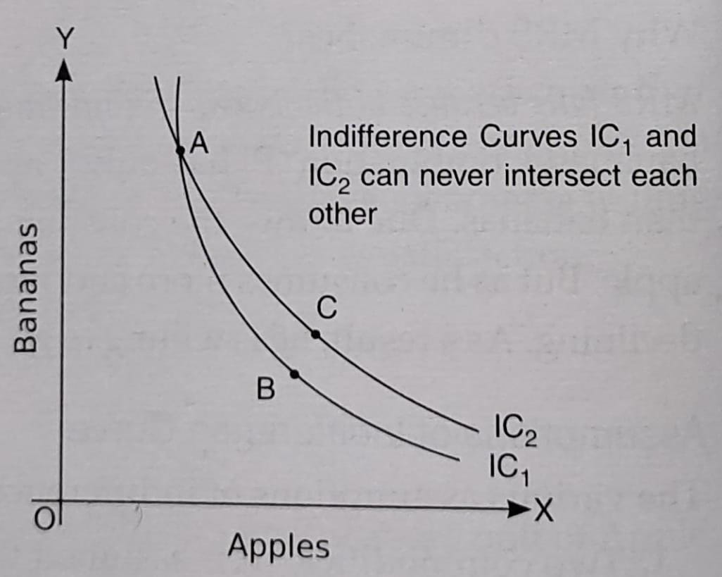
4. Indifference curves can never intersect each other: As two indifference curves cannot represent the same level of satisfaction, they cannot intersect each other. It means, only one indifference curve will pass through a given point on an indifference map. In Fig. 1.5, satisfaction from point A and from B on IC₁ will be the same. Similarly, points A and C on IC₂ also give the same level of satisfaction. It means, points B and C should also give the same level of satisfaction. However, this is not possible, as B and C lie on two different indifference curves, \(IC_1\) and \(IC_2\) respectively and represent different levels of satisfaction. Therefore, two indifference curves cannot intersect each other.
An Indifference Curve can never touch X-axis or Y-axis
- The Indifference Curve analysis assumes consumption of two goods, ie. two goods are always consumed. If indifference curve touches Y-axis, it would mean that consumption of commodity on the X-axis is zero.
- Similarly, if indifference curve touches X-axis, it would mean that consumption of commodity on the Y-axis is zero.
So, an indifference curve can never touch any of the axes.
CONSUMER’S EQUILIBRIUM BY INDIFFERENCE CURVE ANALYSIS
Consumer equilibrium refers to a situation, in which a consumer derives maximum satisfaction, with no intention to change it and subject to given prices and his given income. The point of maximum satisfaction is achieved by studying indifference map and budget line together.
On an indifference map, higher indifference curve represents a higher level of satisfaction than any lower indifference curve. So, a consumer always tries to remain at the highest possible indifference curve, subject to his budget constraint.
Conditions of Consumer’s Equilibrium
The consumer’s equilibrium under the indifference curve theory must meet the following two conditions:
(i) \(MRS_{xy}\)= Ratio of prices or \(\frac{P_x}{P_y}\)
Let the two goods be X and Y. The first condition is that \(MRS_{xy}\) = \(\frac{P_x}{P_y}\)
- If \(MRS_{xy}\) > \(\frac{P_x}{P_y}\), it means that to obtain one more unit of X, Py the consumer is willing to sacrifice more units of Y as compared to what is required in the market. It induces the consumer to buy more of X. As a result, MRS falls and continue to fall till it becomes equal to the ratio of prices and the equilibrium is established.
- If \(MRS_{xy}\) < \(\frac{P_x}{P_y}\), it means that Py to obtain one more unit of X, the consumer is willing to sacrifice less units of Y as compared to what is required in the market. It induces the consumer to buy less of X and more of Y. As a result, MRS rises till it becomes equal to the ratio of prices and the equilibrium is established.
(ii) MRS continuously falls. The second condition for consumer’s equilibrium is that MRS must be diminishing at the point of equilibrium, ie. the indifference curve must be convex to the origin at the point of equilibrium. Unless MRS continuously falls, the equilibrium cannot be established.

Thus, both the conditions need to be fulfilled for a consumer to be in a equilibrium.
Let us now understand this with the help of a diagram:
In Fig. 1.6, \(IC_1\), \(IC_2\) and \(IC_3\) are the three indifference curves and AB is the budget line. With the constraint of budget line, the highest indifference curve, which a consumer can reach, is \(IC_2\). The budget line is tangent to indifference curve \(IC_2\) at point ‘E’. This is the point of consumer equilibrium, where the consumer purchases OM quantity of commodity ‘X’ and ON quantity of commodity ‘Y’.
All other points on the budget line to the left or right of point ‘E’ will lie on lower indifference curves and thus indicate a lower level of satisfaction. As budget line can be tangent to
one and only one indifference curve, consumer maximizes his satisfaction at point E, when both the conditions of consumer’s equilibrium are satisfied:
(1) MRS = Ratio of prices \(\frac{P_x}{P_y}\): At tangency point E, the absolute value of the slope of the indifference curve (MRS between X and Y) and that of the budget line (price ratio) are same. Equilibrium cannot be established at any other point as \(MRS_{xy}\) > \(\frac{P_x}{P_y}\) at all points to the left of point E and \(MRS_{xy}\) < \(\frac{P_x}{P_y}\) at all points to the right of point E. So, equilibrium is established at point E, when \(MRS_{xy}\) = \(\frac{P_x}{P_y}\)
(ii) MRS continuously falls: The second condition is also satisfied at point E as MRS is diminishing at point E, i.e. \(IC_2\) is convex to the origin at point E.
Cardinal Utility Vs Ordinal Utility
- Under cardinal utility approach, it is assumed that utility can be measured in cardinal terms, such as 1, 2, 3, etc. However, according to ordinal utility approach, utility is a subjective concept, which cannot be measured and we can just rank the scale of preferences.
- Under cardinal approach, the term “util” was developed as a unit to measure utility, whereas, no such unit of measurement was developed under ordinal approach.
- Example: Suppose a person consumes apple and banana.
According to cardinal approach, the consumer can assign utils to both the commodities, say, 20 utils to apple and 15 utils to banana. It signifies that apple offers 5 more utils than banana.
According to ordinal approach, the consumer cannot express the satisfaction in exact terms. It means, if the consumer likes apple more than banana, then he will give 1st rank to apple and 2nd rank to banana.
The real elaboration of the Indifference Curves was made by J. R. Hicks and R. G. D. Allen, popularly known as Hicks and Allen. In 1934, they wrote an article, ‘A Reconstruction of the Theory of Value’, presenting the Indifference Curve Analysis.
Modern economists disregarded the concept of ‘cardinal measure of utility’. They were of the opinion that utility is a psychological phenomenon and it is next to impossible to measure the utility in absolute terms. According to them, a consumer can rank various combinations of goods and services in order of his preference.
For example, if a consumer consumes two goods, Apples and Bananas, then he can indicate:
- Whether he prefers apple over banana; or
- Whether he prefers banana over apple; or
- Whether he is indifferent between apples and bananas, i.e. both are equally preferable and both of them give him same level of satisfaction.
This approach does not use cardinal values like 1, 2, 3, 4, etc. Rather, it makes use of ordinall numbers like 1st, 2nd, 3rd, 4th, etc. which can be used only for ranking. It means, if the consumer likes apple more than banana, then he will give 1st rank to apple and 2nd rank to banana. Such a method of ranking the preferences is known as ‘ordinal utility approach’. Ordinal utility is the utility expressed in ranks.
Before we proceed to determine the consumer’s equilibrium through this approach, let us understand some useful concepts related to Indifference Curve Analysis.
Meaning of indifference Curve
When a consumer consumes various goods and services, then there are some combinations, which give him exactly the same total satisfaction. The graphical representation of such combinations is termed as indifference curve.
Indifference curve refers to the graphical representation of various alternative combinations of bundles of two goods among which the consumer is indifferent.
Alternately, indifference curve is a locus of points that show such combinations of two commodities which give the consumer same satisfaction. Let us understand this with the help of following indifference schedule, which shows all the combinations giving equal satisfaction to the consumer.
Table 1.3 Indifference Schedule
| Combination of Apples and Bananas | Apples (A) | Bananas (B) |
|---|---|---|
| P | 1 | 15 |
| Q | 2 | 10 |
| R | 3 | 6 |
| S | 4 | 3 |
| T | 5 | 1 |
As seen in the schedule, consumer is indifferent between five combinations of apple and banana. Combination ‘P’ (1A + 15B) gives the same utility as (2A + 10B), (3A + 6B) and so on. When these combinations are represented graphically and joined together, we get an indifference curve ‘IC₁’ as shown in Fig. 2.4.
In the diagram, apples are measured along the X-axis and bananas on the Y-axis. All points (P, QR. S and T) on the curve show different combinations of apples and bananas. These points are joined with the help of a smooth curve, known as indifference curve (IC₁’). An indifference curve is the locus of all the points, representing different combinations, that are equally satisfactory to the consumer.
Every point on IC₁ represents an equal amount of satisfaction to the consumer. So, the consumer is said to be indifferent between the combinations located on Indifference Curve IC₁.
The combinations P, Q, R, S and T give equal satisfaction to the consumer and therefore he is indifferent among them. These combinations are together known as ‘Indifference Set’.
Monotonic Preferences
Monotonic preference means that a rational consumer always prefers more of a commodity as it offers him a higher level of satisfaction. In simple words, monotonic preferences implies that as consumption increases total utility also increases. For instance, a consumer’s preferences are monotonic only when between any two bundles, he prefers the bundle which has more of at least one of the goods and no less of the other good as compared to the other bundle.
Example: Consider 2 goods: Apples (A) and Bananas (B).
- Suppose two different bundles are: 1st: (10A, 10B); and 2nd: (7A, 7B). Consumer’s preference of 1st bundle as compared to 2nd bundle will be called monotonic preference as 1st bundle contains more of both apples and bananas.
- If 2 bundles are: 1st: (10A, 7B); 2nd: (9A, 7B).
Consumer’s preference of 1 bundle as compared to 2nd bundle will be called monotonic preference as 1ª bundle contains more of apples, although bananas are same.
Indifference Map
Indifference Map refers to the family of indifference curves that represent consumer preferences over all the bundles of the two goods.
An indifference curve represents all the combinations, which provide same level of satisfaction. However, every higher or lower level of satisfaction can be shown on different indifference curves. It means, infinite number of indifference curves can be drawn.
In Fig. 1.3, IC₁ represents the lowest satisfaction, IC₁ shows satisfaction more than that of IC₁ and the highest level of satisfaction is depicted by indifference curve IC₁ However, each indifference curve shows the same level of satisfaction individually.
It must be noted that ‘Higher Indifference curves represent higher levels of satisfaction’ as higher indifference curve represents larger bundle of goods, which means more utility because of monotonic preference.
Marginal Rate of Substitution (MRS)
MRS refers to the rate at which the commodities can be substituted with each other, so that total satisfaction of the consumer remains the same. For example, in the example of apples (A) and bananas (B), MRS of ‘A’ for ‘B’, will be number of units of ‘B’, that the consumer is willing to sacrifice for an additional unit of A’ so as to maintain the same level of satisfaction.
\(MRS_{AB}=\frac{Units\;of\;Bananas(B)\;willing\;to\;Sacrifice}{Units\;of\;Apples(A)\;willing\;to\;Gain}\)
\(MRS_{AB}=\frac{ΔB}{ΔA}\)
\(MRS_{AB}\) is the rate at which a consumer is willing to give up Bananas for one more unit of Apple. It means, MRS measures the slope of indifference curve.
It must be noted that in mathematical terms, MRS should always be negative as numerator (units to be sacrificed) will always have negative value. However, for analysis, absolute value of MRS is always considered.
The concept of MRSAB is explained through Table 1.4 and Fig. 1.4.
Table 1.4 MRS between Apple and Banana
| Combination | Apples (A) | Bananas (B) | MRS_AB |
|---|---|---|---|
| P | 1 | 15 | — |
| Q | 2 | 10 | 5B : 1A |
| R | 3 | 6 | 4B : 1A |
| S | 4 | 3 | 3B : 1A |
| T | 5 | 1 | 2B : 1A |
As seen in the given schedule and diagram, when consumer moves from P to Q, he sacrifices 5 bananas for 1 apple. Thus, MRSAB comes out to be 5:1. Similarly, from Q to R, \(MRS_{AB}\) is 4:1. In combination T, the sacrifice falls to 2 bananas for 1 apple. In other words, the MRS of apples for bananas is diminishing.
Why MRS diminishes?
MRS falls because of the law of diminishing marginal utility. In the given example of apples and bananas, Combination ‘P’ has only 1 apple and, therefore, apple is relatively more important than bananas. Due to this, the consumer is willing to give up more bananas for an additional apple. But as he consumes more and more of apples, his marginal utility from apples keeps on declining. As a result, he is willing to give up less and less of bananas for each additional apple.
Assumptions of Indifference Curve
The various assumptions of indifference curve are:
- Two commodities: It is assumed that the consumer has a fixed amount of money, whole of which is to be spent on the two goods, given constant prices of both the goods.
- Non Satiety: It is assumed that the consumer has not reached the point of saturation. Consumer always prefer more of both commodities, i.e. he always tries to move to a higher indifference curve to get higher and higher satisfaction.
- Ordinal Utility: Consumer can rank his preferences on the basis of the satisfaction from each bundle of goods.
- Diminishing marginal rate of substitution: Indifference curve analysis assumes diminishing marginal rate of substitution. Due to this assumption, an indifference curve is convex to the origin.
- Rational Consumer: The consumer is assumed to behave in a rational manner, i.e. he aims to maximise his total satisfaction.
Properties of Indifference Curve
- Indifference curves are always convex to the origin: An indifference curve is convex to the origin because of diminishing MRS. MRS declines continuously because of the law of diminishing marginal utility. As seen in Table 1.4, when the consumer consumes more and more of apples, his marginal utility from apples keeps on declining and he is willing to give up less and less of bananas for each apple. Therefore, indifference curves are convex to the origin (see Fig. 1.4). It must be noted that MRS indicates the slope of indifference curve.
- Indifference curve slope downwards: It implies that as a consumer consumes more of one good, he must consume less of the other good. It happens because if the consumer decides to have more units of one good (say apples), he will have to reduce the number of units of another good (say bananas), so that total satisfaction remains the same.
- Higher Indifference curves represent higher levels of satisfaction: Higher indifference curve represents large bundle of goods, which means more utility because of monotonic preference. Consider point ‘ A’ on IC₁ and point ‘B’ on \(IC_2\) in Fig. 1.3. At ‘A’, consumer gets the combination (OR, OP) of the two commodities x and y. At ‘B’, consumer gets the combination (OS, OP). As OS > OR the consumer gets more satisfaction at \(IC_2\).
4. Indifference curves can never intersect each other: As two indifference curves cannot represent the same level of satisfaction, they cannot intersect each other. It means, only one indifference curve will pass through a given point on an indifference map. In Fig. 1.5, satisfaction from point A and from B on IC₁ will be the same. Similarly, points A and C on IC₂ also give the same level of satisfaction. It means, points B and C should also give the same level of satisfaction. However, this is not possible, as B and C lie on two different indifference curves, \(IC_1\) and \(IC_2\) respectively and represent different levels of satisfaction. Therefore, two indifference curves cannot intersect each other.
An Indifference Curve can never touch X-axis or Y-axis
- The Indifference Curve analysis assumes consumption of two goods, ie. two goods are always consumed. If indifference curve touches Y-axis, it would mean that consumption of commodity on the X-axis is zero.
- Similarly, if indifference curve touches X-axis, it would mean that consumption of commodity on the Y-axis is zero.
So, an indifference curve can never touch any of the axes.
Introduction
The price effect is a fundamental concept in economics that describes how changes in the price of a good or service influence the quantity demanded or quantity supplied. It is a crucial aspect of consumer behavior and market dynamics, forming the basis of many economic theories, including demand and supply analysis.
The price effect can be broken down into two primary components:
- Substitution Effect – Consumers switch between goods based on relative price changes.
- Income Effect – Changes in purchasing power affect the quantity demanded.
Understanding the Price Effect
The price effect occurs because consumers respond to price changes in predictable ways. When the price of a good decreases, consumers are generally willing to purchase more of that good, and when the price increases, they purchase less. This inverse relationship between price and quantity demanded is represented by the law of demand.
On the supply side, firms respond to price changes as well. A higher price typically incentivizes producers to increase supply, while a lower price discourages production. This direct relationship between price and quantity supplied follows the law of supply.
The overall effect of a price change can be decomposed into substitution effect and income effect, both of which explain shifts in consumer demand.
The Substitution Effect
The substitution effect occurs when a change in the price of a good makes it relatively more or less expensive compared to substitutes. As a result, consumers tend to switch their purchases accordingly.
- When the price of a good falls, it becomes relatively cheaper compared to other goods, encouraging consumers to buy more of it instead of its substitutes.
- When the price of a good rises, it becomes relatively more expensive, prompting consumers to shift to cheaper alternatives.
For example, if the price of coffee increases, consumers may switch to tea, assuming both goods serve as substitutes. This effect operates independently of income changes and is purely based on relative prices.
The substitution effect is particularly strong for goods with many close substitutes (e.g., butter and margarine) and weaker for goods with fewer substitutes (e.g., insulin for diabetic patients).
The Income Effect
The income effect explains how a change in price affects a consumer’s real purchasing power.
- If the price of a good falls, consumers effectively feel richer, as their existing income can now buy more of the good than before. This leads to an increase in quantity demanded.
- If the price of a good rises, consumers feel poorer, as their purchasing power declines, leading to a decrease in quantity demanded.
The strength of the income effect depends on whether the good is classified as:
- Normal Goods – Goods for which demand increases as income rises (e.g., organic food, branded clothing).
- Inferior Goods – Goods for which demand decreases as income rises (e.g., instant noodles, public transportation).
For instance, if the price of luxury cars decreases, individuals who previously could not afford them might now be able to purchase one due to the higher real purchasing power. On the other hand, if bus fares decrease, some people might continue using buses instead of switching to taxis, demonstrating an income effect on inferior goods.
Graphical Representation of the Price Effect
Economists use indifference curves and budget constraints to analyze the price effect graphically.
- An indifference curve represents different combinations of two goods that provide equal satisfaction to a consumer.
- A budget constraint shows the various combinations of goods a consumer can afford given their income.
When the price of a good falls:
- The budget constraint shifts outward, allowing the consumer to afford more of both goods.
- The new equilibrium point on the indifference curve reflects the combined substitution and income effects.
This graphical approach helps in understanding how consumer equilibrium is influenced by price changes.


- Substitution & Income Effects – Shows how a consumer’s budget shifts when the price of a good decreases, increasing the quantity demanded.
- Giffen Goods – Depicts an upward-sloping demand curve, where a price increase leads to higher demand (a rare exception to the Law of Demand).
- Veblen Goods – Illustrates how luxury goods defy the normal price effect, as higher prices attract more consumers due to prestige.
- Elastic vs. Inelastic Demand – Compares demand elasticity, showing how different goods respond to price changes.
Giffen and Veblen Goods: Exceptions to the Price Effect
Giffen Goods (A Special Case of Inferior Goods)
Giffen goods are an exception to the typical price effect where an increase in price leads to an increase in quantity demanded instead of a decrease. This occurs when:
- The good is a strongly inferior good, meaning the income effect outweighs the substitution effect.
- The good is a staple commodity, making up a large portion of consumer expenditure.
For example, during economic hardships, if the price of staple foods like rice or bread rises, lower-income consumers might be forced to spend even more on these goods by reducing expenditures on other items. This paradox was first observed by economist Sir Robert Giffen.
Veblen Goods (Luxury Goods and Status Symbols)
Veblen goods defy the price effect due to their prestige value. A higher price increases their attractiveness because they are seen as a status symbol.
Examples include:
- Luxury watches (e.g., Rolex)
- Designer clothing (e.g., Gucci, Louis Vuitton)
- High-end cars (e.g., Ferrari, Rolls-Royce)
For Veblen goods, the higher price itself is a selling point, as it signals exclusivity and wealth. The demand curve for such goods slopes upward instead of downward.
Price Elasticity of Demand and the Price Effect
The strength of the price effect depends on a concept called price elasticity of demand (PED), which measures how sensitive quantity demanded is to price changes.
- Elastic Demand (|PED| > 1): A small price change leads to a large change in quantity demanded. Example: Electronics, luxury items.
- Inelastic Demand (|PED| < 1): A price change has little effect on quantity demanded. Example: Necessities like salt, medicine.
- Unitary Elastic Demand (|PED| = 1): Proportional response of quantity demanded to price changes.
If demand is elastic, the price effect is strong, meaning price cuts significantly boost sales. If demand is inelastic, price changes have minimal impact on consumption.
Implications of the Price Effect in Market Economy
- Business Pricing Strategies – Companies analyze price effects when setting prices for products. A firm selling an elastic good may lower prices to increase revenue, whereas a firm selling an inelastic good may raise prices without fearing a drop in demand.
- Government Policy – Policymakers use price effect insights for taxation and subsidies. Higher taxes on cigarettes reduce smoking due to price-sensitive demand. Conversely, subsidies on public transport encourage usage.
- Consumer Behavior and Welfare – Price effects determine consumer surplus, which is the difference between what consumers are willing to pay and what they actually pay. Lower prices increase consumer surplus, improving overall welfare.
Conclusion
The price effect is a crucial economic concept explaining how price changes impact consumer choices. It consists of the substitution effect, where consumers switch between goods, and the income effect, which alters purchasing power. While most goods follow the law of demand, exceptions like Giffen and Veblen goods challenge conventional patterns. Furthermore, price elasticity of demand plays a key role in determining the strength of the price effect. Understanding the price effect helps businesses, policymakers, and economists predict consumer behavior and design effective strategies in a market-driven economy.
The income effect, in microeconomics, is the resultant change in demand for a good or service caused by an increase or decrease in a consumer’s purchasing power or real income. As one’s income grows, the income effect predicts that people will begin to demand more (and vice-versa).
So-called normal goods will exhibit this typical pattern. Inferior goods, on the other hand, may see their demand actually fall as income increases. An example of such an inferior good could be store-brand items: as people become wealthier they may opt instead for more expensive name brands,
Key Takeaways
The income effect describes how an increase in income can change the quantity of goods that consumers will demand.
For so-called normal goods, as income rises so does the demand for them (and vice-versa).
This is reflected in microeconomics via an upward shift in the downward-sloping demand curve.
This effect, however, can vary depending on the availability of substitutes and the good’s elasticity of demand.
For inferior goods, the income effect dominates the substitution effect and leads consumers to purchase more of a good, and less of substitute goods, when the price rises.
Understanding the Income Effect
The income effect is a part of consumer choice theory—which relates preferences to consumption expenditures and consumer demand curves—that expresses how changes in relative market prices and incomes impact consumption patterns for consumer goods and services. For normal economic goods, when real consumer income rises, consumers will demand a greater quantity of goods for purchase.
The income effect and substitution effect are related economic concepts in consumer choice theory. The income effect expresses the impact of changes in purchasing power on consumption, while the substitution effect describes how a change in relative prices can change the pattern of consumption of related goods that can substitute for one another.
Changes in real income can result from nominal income changes, price changes, or currency fluctuations. When nominal income increases without any change to prices, this means consumers can purchase more goods at the same price, and for most goods, consumers will demand more.
If all prices fall, known as deflation and nominal income remains the same, then consumers’ nominal income can purchase more goods, and they will generally do so. These are both relatively straightforward cases. However in addition, when the relative prices of different goods change, then the purchasing power of consumer’s income relative to each good changes—then the income effect really comes into play. The characteristics of the good impact whether the income effect results in a rise or fall in demand for the good.
When the price of a product increases relative to other similar products, consumers will tend to demand less of that product and increase their demand for the similar product as a substitute.
Normal Goods vs. Inferior Goods
Normal goods are those whose demand increases as people’s incomes and purchasing power rise. A normal good is defined as having an income elasticity of demand coefficient that is positive, but less than one.
For normal goods, the income effect and the substitution effect both work in the same direction; a decrease in the relative price of the good will increase quantity demanded both because the good is now cheaper than substitute goods, and because the lower price means that consumers have a greater total purchasing power and can increase their overall consumption.
Inferior goods are goods for which demand actually declines as consumers’ real incomes rise, or rises as incomes fall. This occurs when a good has more costly substitutes that see an increase in demand as the economy improves. For inferior goods, the income elasticity of demand is negative, and the income and substitution effects work in opposite directions.
An increase in the inferior good’s price means that consumers will want to purchase other substitute goods instead but will also want to consume less of any other substitute normal goods because of their lower real income.
Inferior goods tend to be goods that are viewed as lower quality, but can get the job done for those on a tight budget, for example, generic bologna or coarse, scratchy toilet paper. Consumers prefer a higher quality good, but need a greater income to allow them to pay the premium price.
Example of Income Effect
Consider a consumer who on an average day buys a cheap cheese sandwich to eat for lunch at work, but occasionally splurges on a luxurious hot dog. If the price of a cheese sandwich increases relative to hotdogs, it may make them feel like they cannot afford to splurge on a hotdog as often because the higher price of their everyday cheese sandwich decreases their real income.
In this situation, the income effect dominates the substitution effect, and the price increase raises demand for the cheese sandwich and reduces demand for a substitute normal good, a hotdog, even if the hotdog’s price remains the same.
What Does the Income Effect Depict?
The income effect is a part of consumer choice theory—which relates preferences to consumption expenditures and consumer demand curves—that expresses how changes in relative market prices and incomes impact consumption patterns for consumer goods and services. In other words, it is the change in demand for a good or service caused by a change in a consumer’s purchasing power resulting from a change in real income. This income change can be the result of a rise in wages etc., or because existing income is freed up by a decrease or increase in the price of a good that money is being spent on.
What Is the Difference Between the Income Effect and the Price Effect?
The difference between the income effect and the price effect is that the income effect evaluates consumer spending habits based on a change in their income. The price effect instead considers consumer spending habits based on a change in the price of a good or service.
What Is Substitution Effect?
The substitution effect is the decrease in sales for a product that can be attributed to consumers switching to cheaper alternatives when its price rises. A product may lose market share for many reasons, but the substitution effect is purely a reflection of frugality. If a brand raises its price, some consumers will select a cheaper alternative.
What Are Normal Goods?
Normal goods are those whose demand increases as people’s incomes and purchasing power rise. As such, a normal good will have a positive income elasticity of demand coefficient but it will be less than one. This means that a decrease in the relative price of the good will result in an increase in quantity demanded both because the good is now cheaper than substitute goods, and because the lower price means that consumers have a greater total purchasing power and can increase their overall consumption.
What Are Inferior Goods?
Inferior goods are goods for which demand declines as consumers’ real incomes rise, or rises as incomes fall. Consumers with more money may opt to buy more expensive substitutes instead of what they could afford only when incomes were lower.
The Bottom Line
The income effect identifies the change in consumers’ demand for goods and services based on their incomes. In general, as one’s income rises, they will begin to demand more goods. Similarly, A decrease in income results in lower demand. The marginal propensity to spend and the marginal propensity to save are looked at when determining the influences of the income effect. The substitution effect also plays a role in how consumers spend their income in times of rising or declining income. For normal goods the income effect works as predicted. For inferior goods, it works in the opposite direction.
Revealed Preference Theory (RPT) is an economic concept that gauges consumer preferences based on the goods they purchase under various price and income scenarios. It was developed to reconcile the utility and demand theories by analyzing customers’ behavior through utility functions.

Revealed preference theory
The belief that customers act rationally roots the foundation of the theory. By holding the price of goods and customers’ income constant, one can determine their purchasing preferences. The theory is best understood through the Weak Axiom of Revealed Preference (WARP), Strong Axiom of Revealed Preference (SARP), and Generalized Axiom of Revealed Preference (GARP).
Revealed preference theory is an economic model to uncover individual preferences based on observed buying patterns.
Revealed preference theory provides a useful tool for analyzing and predicting consumer behavior, particularly regarding how consumers react to price changes and income levels.
It reconciles the utility concept with demand theory by assuming customer choices reflect their preferences. The theory assumes constant prices, incomes, and consistent consumer tastes over time.
Researchers have identified eight main limitations of the theory, including the fact that individual choices may not always reflect true preferences.
Revealed Preference Theory in Economics
Revealed preference theory’s axioms provide a systematic framework for analyzing and evaluating consumer choices, allowing businesses and policymakers to make informed decisions based on consumer behavior patterns. By understanding customers’ preferences, companies can better tailor their products and services to meet their needs, increasing sales and customer satisfaction. It, thus, is essential for understanding consumer preferences by examining their purchasing behavior.
In 1938, economist Paul Anthony Samuelson developed the theory of RPT to quantify the revealed preference theory of consumer behavior. Samuelson illustrated that if a person is given two commodities to choose from (A & B) and two combinations of these commodities (X & Y) with the same quality and price, the person will choose the combination (X) over (Y) because they prefer it.
The price line represents the customer’s real income-price situation, and the consumer may choose any combination on or to the left of the price line, creating a choice triangle from which they can buy any goods. Consumers consider combinations on the price line equally desirable, deem combinations below the price line inferior, and consider those above the price line superior. The difference between the preferred and inferior zones is known as the ignorance zone.
In summary, RPT provides an essential framework for analyzing consumer behavior and understanding their preferences by examining their purchasing decisions at different prices and income levels.
Assumptions
Assumptions of revealed preference theory:
- Consumer tastes remain constant over time.
- The choices a consumer makes reveal their preferences.
- On a price-income line, the consumer selects only one combination.
- Consumers prefer larger sets of goods to smaller ones.
- Consumers have complete and transitive preferences, meaning that if A is preferred over B, and B is preferred over C, then A is preferred over C.
- Consumer behavior exhibits consistency over time.
- Consumers demand more goods as their income increases and less as their income decreases.
- A consumer will purchase more of a product if the price drops significantly.
Diagram
Let us look into the diagrammatic representation of revealed preference theory:
 The revealed preference theory is a way of understanding people’s preferences based on their observable behavior, such as buying decisions. People often depict the theory graphically using a simple budget constraint diagram.
The diagram consists of two axes: the horizontal axis represents the quantity of one good, and the vertical axis represents the quantity of another good. The budget constraint is a straight line that shows all the combinations of the two goods that can occur with a given income level and the prices of the goods. The slope of the budget constraint represents the relative prices of the two goods.
The area under the budget constraint represents all the available feasible consumption bundles, given the income level and prices of the goods. Any point on the budget constraint represents a particular consumption bundle that exhausts the consumer’s income. The area above the budget constraint represents unaffordable consumption bundles, given the income level and prices of the goods.
Overall, the revealed preference theory graph provides a visual representation of how consumers choose to allocate their limited income among different goods based on their preferences and the prices of the goods.
Limitations
Despite its merits, like being realistic, scientific, consistent, and based on minimal assumptions, the revealed preference theory has faced some criticism. The limitations of RPT theory are the following:
- It does not account for the possibility of indifferences in consumer behavior.
- It fails to distinguish between the income and substitution effect of a price change.
- It only derives the demand curve of an individual and not the market demand curve.
- It considers the consumer behavior of only individuals governed by existing market conditions.
- RPT does not consider that consumers can choose from multiple combinations instead of only one.
- The choice made by the consumer does not necessarily reflect their true preference.
- Game theory becomes invalid under RPT.
- RPT tends to fail in risky or ambiguous situations.
Introduction
consumer’s surplus was introduced in economics by Alfred Marshall, although the use of the concept goes back at least to the Freanch economist Dupuit writing in the first half of the nineteenth century.
Two Nobel Prize winners in economics disagree fundamentally about the utility of the concept; John Hicks saw great use for the concept as a cornerstone of welfare economics, whereas Paul Samuelson believes that we can talk of discard the concept without loss. There is also the question of whether we can talk of consumer’s surplus or only of consumer’s surplus—whether we can use the concept for a whole group of consumers of a product or only for an individual household.
The doctrine of consumer’s surplus is a deduction from the law of diminishing marginal utility. The price that we pay for a thing measures only the marginal utility, but not the total utility. Only on the marginal unit, which a man is just induced to buy, the price is exactly equal to the satisfaction that he expects to get from that unit. But, on other units that he buys, he enjoys some extra amount of satisfaction.
He would be willing to pay higher prices for these units than what he actually pays for them. The difference between the amount of satisfaction which a consumer obtains from purchasing things over that which he actually pays for them is the economic measure of consumer’s surplus.
It represents the excess of satisfaction that he secures, the excess being equal to the difference between the utility of the goods acquired and that of the money sacrificed. Had he been deprived of the commodity, he would then have been forced to spend the money on the purchase of other commodities from which he does not derive the same amount of satisfaction, but less.
Alfred Marshall has introduced the term ‘consumer’s surplus’ in economic theory to show that, in various situations consumer receives more from a commodity than he pays for it.
Marshall explained consumer’s surplus thus:
“The price which a person pays for a thing can never exceed and seldom comes up to that which he would be willing to pay rather than go without it – so that the satisfaction which he gets from its purchase generally exceeds that which he gives up in paying away its price: and he thus derives from the purchase a surplus of satisfaction”.
The excess of the price which he would be willing to pay rather than go without the thing, over that which he actually does pay, is the economic measure of this surplus satisfaction. In short, the benefit which a person derives from purchasing, at a low price, thing for which he would rather pay a high price, than go without it may be called his consumer’s surplus.
At times, we find that a consumer’s willingness to pay for a commodity may be greater than the price he actually pays for it. The price that he is ready to pay for a commodity is his individual demand price and the price he actually pays for it is the market price. According to Paul Samuelson, consumer’s surplus is nothing but the excess of the individual demand price over the market price of a commodity (or, the positive difference between the potential price and the actual price of a commodity).
Example:
In order to give definiteness to our idea, let us take the example of shoes. Suppose, from the first pair of shoes a man expects to get satisfaction worth at least Rs. 500, from the second he expects additional satisfaction worth Rs. 400, from the third he expects additional satisfaction worth Rs. 300. Suppose, he is just induced to buy three pairs and no more.
Since in a market there cannot be more than one price, the price that he pays for each pair is measured by that of the marginal pair, i.e., by Rs. 300. He will pay (Rs. 300 x 3) or Rs. 900 in all for the three pairs. But, by hypothesis, he is enjoying from the three pairs an amount of satisfaction worth (Rs. 500 + Rs. 400 + Rs. 300) = Rs. 1200.
Hence, he enjoys a surplus of satisfaction from his purchase worth (Rs. 1200 – Rs. 900) = Rs. 300. Consumer’s surplus is then measured by the difference between the total utility and the total expenditure made by the consumer on a commodity (shoes). It is the difference between individual demand price and market price.
Hence, the consumer’s surplus may be shown in another way:
Consumer’s Surplus = Total Utility – (Total units purchased x marginal utility or price). In short, consumer’s surplus is the positive difference between the total utility from a commodity and the total payments made for it.
The concept of consumer’s surplus can also be illustrated with the help of Fig. 3:
In Fig. 3, the quality of a particular commodity is measure on the horizontal axis and its marginal utility or production on the vertical axis. Here DD’ is the demand price for it. If a consumer buys all the units (OR) at RS price per unit, he gets a total satisfaction equal to the area DORS. But, he spends only ORST amount of money, so his surplus satisfaction is DTS (i.e., the shaded area). If the price falls to R’ S’, he would buy OR’ and his surplus would increase to DTS’.
So, consumer’s surplus is measured by the area under the demand curve but above the market price. A difficulty is that as the price falls the demand where, the real income of the consumer increases. To get a more accurate measure of the benefit of the surplus; therefore, an adjustment must be made to offset the effect of the difference in real income at the higher price (RS) and the lower price (R’S’).
Difficulties of Measurement
Consumer’s surplus is measured by the area under an individual’s demand curve between two prices. It is a monetary measure, although originally represented in terms of surplus utility by Marshall. It is a measure of the benefit to the consumer, net of the sacrifice he has to make from being able to buy a commodity at a particular price. However, Marshall’s doctrine of consumer’s surplus is subject to a number of criticisms, mainly due to various difficulties associated with this measurement.
The main criticisms of the doctrine are the following:
Constant Marginal Utility of Money
Marshall’s doctrine of consumer’s surplus is based on the assumption of constant marginal utility of money. Hicks considers this to be the greatest difficulty in accepting the concept of consumer’s surplus. As he put it, “A stronger incentive will be required to induce a person to pay a given price for anything if he is poor than if he is rich. A pound is the measure of the less pleasure, or satisfaction, of any kind, to a rich man than to a poor one.”
When a consumer buys more of a particular thing, his stock of money falls and the marginal utility of money to him will increase. Such a reduction in the marginal utility of money will automatically involve the revaluation of the utilities from the earlier units of the commodity!
It is true that Marshall’s assumption of constant marginal utility of money becomes valid when a consumer spends a very small proportion of his income for a commodity. But, this assumption is not always realistic, for a consumer is often required to spend a large portion of his income for a commodity (e.g., expenditure on foodstuff by a poor household).
Lack of Precise Measurement
The accurate measurement of consumer’s surplus is not possible as we have no knowledge of the potential prices that a consumer is willing to pay for the earlier units of the commodity purchased. In fact, the individual demand prices for the earlier units of the commodity are merely hypothetical and imaginary. For this reason, Prof. Nicholson remarks that the concept of consumer’s surplus is purely hypothetical and more a figment than a fact.
Difficulties in Measuring Consumer’s Surplus
Further difficulties arise when we try to increase of consumer’s surpluses of a group or of a community by means of adding up the consumer’s surplus of different individuals. Such difficulties arise because the individual demand price for a thing varies from person to person owing to differences in their incomes, tastes, preferences, etc.
Unlimited Consumer’s Surplus in the Case of Necessities
It is also pointed out that the consumer’s surplus cannot be measured in the case of necessaries and of conventional necessaries of life as their utility (or the individual demand prices for these goods) is infinite or indefinite to a consumer. It is very often found that a consumer is sometimes willing to pay anything under his possession for these goods when he is in urgent need of them, and this makes the individual demand prices for these goods to be infinite. Examples of such goods are textbooks or life-saving drugs.
Conspicuous Consumption Goods
Tausig has pointed out that the concept of consumer’s surplus cannot be applied in the case of articles of conspicuous consumption (e.g., for coats of diamonds). The term was used by Thorstesin Veblem (1857-1929) to identify that ostentatious personal expenditure which satisfies no physical need but rather a psychological need for the esteem of others.
Goods may be purchased not for their practical use but as ‘status symbols’ and to ‘keep up with the Joneses’. These goods have a high prestige value to their users, but their utility falls when their prices fall. In such cases, a fall in the prices causes a fall in consumer’s surplus — a result which becomes inconsistent with the definition of consumer’s surplus.
Impossibility of Meaning Cardinal Utility
Furthermore, Marshall’s analysis of consumer’s surplus is based on an important premise that the utility of a thing can be measured and numbered. But, most of the modern writers have shown that utility, being a psychological concept, cannot be cardinally (objectively) measured and quantified.
Difficulties in the Case of Complements and Substitutes
Again, consumer’s surplus cannot be measured in the case of complementary goods (e.g., tea and coffee, etc.) Because, in such cases the utility of a thing depends not only on its total stock but also on the supply of other related goods. Marshall has tried to overcome this difficulty by suggesting that we should treat the related goods as one commodity and group them under one common demand schedule. But, actually, it is not possible to do so.
Purely Hypothetical and Unreal Concept
Prof. Nicholson has expressed serious doubts about the utility of the whole doctrine. He asked, “Of what avail is it to say that the utility of an income of (say) £ 100 a year is worth (say) £ 1000 a year?” According to him, the doctrine is thus purely hypothetical and unreal.
But, Marshall points out that the question raised by Nicholson would have some relevance if we compare the living conditions in Central Africa with those in London. There are many things, many amenities of life which are available in London, but not in Central Africa. The living conditions at those two places may be measured by the statement that £ 100 in London yields the same benefits to the consumer as £ 1000 in Central Africa.
Useless Theoretical Toy
Prof. Little has characterised the concept of consumer’s surplus as “a totally useless theoretical toy” as it cannot provide us any practical objective criterion for measuring economic welfare.
Historical and Doctrinal Interest
Samuelson has not attached much importance to the doctrine of consumer’s surplus in the study of economics. He remarks, “The subject (the concept of consumer’s surplus) is of historical and doctrinal interest, with a limited amount of appeal as a mathematical puzzle”.
Hicks’s Concept of consumer’s surplus:
Owing to various difficulties in measuring consumer’s surplus as explained by Marshall, J.R. Hicks has formulated the concept of consumer’s surplus in a different way. In his opinion, “the best way of looking at consumer surplus is to regard it as a means of expressing, in terms of money income, the gain which accrues to the consumer as a result of a fall in price”.
Thus, when a thing (say, sugar or edible oil) becomes cheaper as a result of a fall in its price, a consumer gets the same amount at a lower price. Because of such a gain in money income, he may buy more of that thing or he may buy another thing; in any case he is now better off than before. To Hicks such a gain in money income as a result of a fall in the price of a thing is consumer’s surplus.