The economists like Ricardo, J. S. Mill, Marshall and Pigou developed the, classical theory of interest which is also known as the capital theory of interest or the saving-investment theory of interest or the real theory of interest. According to this theory, interest is a real phenomenon and the rate of interest is determined exclusively by the real factors, i.e., the supply of and demand for capital under perfect competition. The supply of capital is governed by thrift (i.e. saving) or time preference and the demand for capital is influenced by the productivity of capital.

Assumptions of Classical Theory of Interest

The classical theory of interest is based upon the following assumptions:

(i) Perfect competition exists in the factor market.

This assumption has the following implications:

(a) The equilibrium rate of interest is determined by the competitive forces of demand and supply in the capital market.

(b) Interest rate is flexible, i.e., it freely moves to whatever level the demand and supply forces dictate.

(ii) The theory assumes full employment of resources.

This assumption has the following implications:

(a) Saving involves sacrifice of abstaining from or postponing of consumption and interest is the reward for abstinence or waiting: it is only when all resources are fully employed, higher rate of interest is paid to induce people to save or abstain from consumption or postpone consumption

(b) Income level is assumed to be constant; it is at the full employment level that income and output do not change and become constant.

(c) The assumptions of full employment and given level of income lead to the further assumption that the demand and supply schedules of capital are independent and do not influence each other; it is only when income changes as a result of a change in investment, that saving changes in consequence.

(iii) Economic agents act rationally, i.e., they are motivated by self-interest and want to maximise economic benefit.

(iv) The price level is assumed to be constant. If it changes then the economic agents do not suffer money illusion, i.e., savers and investors react to changes in the real interest rates and not the changes in the money interest rates.

(v) Money is neutral and serves only as a medium of exchange and not as a store of value.

Supply and Demand for Capital

Supply of Capital

The supply of capital depends upon savings which, in turn, depend upon a number of psychological, economic and institutional factors broadly classified as – (a) the will to save, (b) the power to save, and (c) the facilities to save. Saving means curtailment of consumption or postponement of the present consumption. Thus, saving involves a sacrifice, abstinence or waiting. The rate of interest is considered to be the reward for abstinence or waiting.

It is an inducement for the act of saving or foregoing the present consumption. In deciding between the present consumption (which involves no saving) and the future consumption (which requires saving), the individual has to take into consideration the opportunity cost of each alternative and the opportunity cost is measured by the rate of interest.

For example, if the current rate of interest is 5% then by consuming Re. 1 of income now, the individual is foregoing the consumption of Rs. 1.05 one year later. Thus, the higher the current rate of interest, the greater the opportunity cost of present consumption as compared to the future consumption, and, as a result, greater the inducement to save out of the present income.

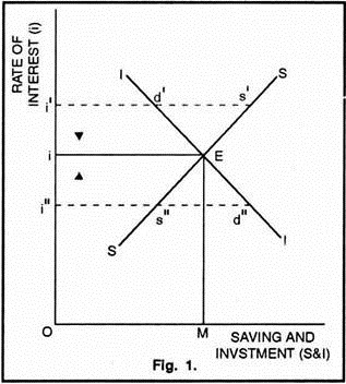
Hence, saving is interest elastic and there is a positive relationship between the rate of interest and saving. The supply curve of capital or the saving schedule (SS curve in Figure 1) slopes upward to the right which indicates that higher the rate of interest, larger will be the savings and greater will be the supply of capital and vice versa.

Demand for Capital

Capital is demanded by the investors because it is productive and brings profits to them. The demand for capital or investment demand depends, on the one hand, on the productivity of capital, i.e., returns on investment, and on the other hand, on the rate of interest, i. e., the cost of investment. Productivity of capital is subject to the law of diminishing returns.

Additional units of capital are less productive than the earlier units; with the investment of more and more capital, the marginal productivity of capital declines. The producer will continue his investment of capital as long as the productivity of capital is more than the rate of interest and will stop further investment when the productivity of capital equals the rate of interest. This shows that at higher rates of interest, the producers demand less capital and at lower rates of interest, they demand more capital.

Thus, the demand for capital is inversely related to the rate of interest. The demand curve for capital or the investment schedule (II curve in Figure I) slopes downward to the right which indicates that higher the rate of interest, smaller the demand for capital.

Determination of Rate of Interest

Assuming the income level to be given, the rate of interest is determined by the intersection of the demand curve and the supply curve of capital.

The determination of equilibrium rate of interest of the following three conditions:

(i) The supply of capital or saving is an increasing function of the rate of interest:

S = f (i); dS/di > 0

(ii) The demand for capital or investment is a decreasing function of the rate of interest:

I = f(i); dl/di < 0

(iii) The supply of capital equals the demand for capital:

S = I

Where, S = saving, I = investment,

and i = rate of interest.

In Figure 1, the II curve (demand curve for capital) intersects the SS curve (supply curve of capital) at point E. The equilibrium rate of interest is Oi and OM is the quantity of capital demanded and supplied at this rate. In other words, at the equilibrium rate of interest, i.e., Oi, saving = investment = OM.

Any deviation from the equilibrium rate of interest (Oi) will be unstable. If, at any time, the rate of interest rises to Oi the supply of capital exceeds the demand for capital (i s’ > id’). As a result of this excess of capital supply, the rate of interest will fall to its equilibrium level (Oi). Similarly, if the rate of interest falls to Oi”, the demand for capital exceeds the supply of capital (i” d” > i” s”). As a result of this excess of capital demand, the rate of interest rises to its equilibrium level (Oi).

Features of Classical Theory

The distinguishing features of the classical theory of interest are given below:

1. Capital Theory of Interest:

In the classical theory, interest is defined as reward for the use of capital and the rate of interest is determined by the demand and supply of capital. The supply of capital is a positive and the demand for capital is a negative function of the rate of interest.

2. Real Theory:

The classical theory is concerned with the real rate of interest which is determined purely by the real factors of saving and investment. The concept of real rate of interest can be defined as the money or market rate of interest less the anticipated rate of inflation. If it is assumed (as the classical theory does) that the price level is constant and everyone anticipates that it will remain constant, then the real and money rates of interest are equal.

3. Flow Theory:

The theory is stated in flow terms. Total saving and total investment have been considered as flows per unit of time. In other words, the supply of saving is regarded as a flow of funds into the capital market and the demand for investment as a flow of funds off the capital market. The equilibrium of the capital market requires the equilibrium between the flows of saving and investment.

4. Equilibrating Mechanism:

According to the classical theory, the rate of interest is the equilibrating force between saving and investment. Whenever there is disequilibrium between saving and investment, the equilibrium is restored through changes in the rate of interest. If at any time, saving exceeds investment (i’ s’ > i’ d’ at Oi’ rate of interest in Figure I), the rate of interest falls and brings equality between saving and investment. On the other hand, if investment exceeds saving (i” d” > i” s” at Oi” rate of interest), the rate of interest rises and brings equality between saving and investment.

5. Positive Rate of Interest:

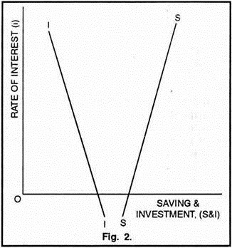
An important feature of the classical theory of interest is that it assumes a positive real rate of interest. The theory implicitly requires that the demand and supply curves of capital intersect at a positive real rate of interest. If, for example, the two curves do not intersect at a positive rate of interest (as shown in Figure 2), then, at zero rate of interest, there will be excess supply of capital (Os > Od). This is a situation of general glut which implies that equilibrium is inconsistent with fill employment.

Criticisms of Classical Theory

The classical theory of interest has been criticized by Keynes on many grounds:

1. Interest not a Reward for Saving:

Keynes has criticized the classical view that interest is the reward for saving or capital on the following grounds:

(a) An individual can get interest by lending money which he has not saved but has inherited from his forefathers.

(b) If a person hoards his savings in the form of cash, he earns no interest,

(c) Savings depend not only on the rate of interest but also on the level of income, hence interest cannot be a reward for saving,

(d) Keynes regards interest as a monetary phenomenon and defines the rate of interest as a reward for parting with liquidity (or cash balances) rather than a reward for saving.

2. Saving and Investment not Interest Elastic:

The classical theory assumes that saving and investment are interest elastic, i.e., sensitive to changes in the rate of interest. But it is not always so. In reality, investment depends more on marginal efficiency of capital and future expectations than on the rate of interest, particularly during periods of depression.

Similarly, savings are rarely interest elastic. People may save without any rise in the rate of interest, or may save even if the rate of interest falls to zero. In fact, savings are more influenced by the level of income than by the rate of interest.

3. Rate of Interest not Equilibrating Force:

According to the classical economists, the equality between saving and investment is maintained by the interest rate adjustment mechanism. Keynes objected to this view and gave a different mechanism for restoring the equality. According to him, income, and not rate of interest, is the equilibrating force between saving and investment. Whenever saving exceeds investment, income level declines. As a result, saving falls and becomes equal to investment. Similarly, if investment exceeds saving, income level rises, saving increases and becomes equal to investment.

4. Role of Money Ignored:

The classical theory of interest assumes money to be neutral, merely acting as a medium of exchange. It ignores the role of money as a store of value, i.e., it does not take in to consideration the possibility that saving may be hoarded. It also completely ignores the important role the quantity of money, the created money and the bank credit can play in the determination of the rate of interest. All these factors make the classical theory unrealistic and irrelevant in the modern dynamic world.

5. Unrealistic Assumption of Full Employment:

The classical theory is unrealistic because it operates under the special conditions of full employment. Normally, less-than full employment, and not full employment, conditions prevail in the actual world. According to Keynes, when there are unemployed resources in the economy, people need not be paid for abstaining from consumption (i.e., for saving). The problem in such an economy is to put idle resources to use rather than to withdraw already employed resources from their existing employment. Hence, under unemployment conditions, interest cannot be a reward for abstinence or waiting.

6. Discrepancy between Market and Natural Rates:

The classical economists assume that discrepancy between the natural (real) and market (money) rates of interest is merely a chance and cannot exist for a long time. But, according to Wicksell, Keynes and other monetary economists, the market rate of interest normally deviates from the natural rate of interest and this deviation is due to the influence of monetary factors like creation and destruction of bank credit.

7. Narrow View of Supply of Capital:

The classical economists included only saving in the supply of capital. But in reality, the supply of capital comprises of dishoarded money. Moreover, newly created money and bank credit also form important sources of supply of capital.

8. Narrow View of Demand for Capital:

According to the classical theory, the demand for capital comes only from the investors for meeting investment expenditures. It completely ignores the fact that loans are also taken for consumption purposes.

9. Indeterminate Theory:

Keynes criticised the classical theory of investment on the ground that it is indeterminate. According to the classical theory, the rate of interest is determined by the intersection of saving and investment curves. The position of the saving curve depends upon the level of income; saving curve shifts to the right if income increases and vice versa.

Thus, we cannot know the rate of interest unless we already know the income level. But, we cannot know income level without first knowing the volume of investment and the knowledge of the volume of investment requires the prior knowledge of the rate of interest. Thus, the classical theory of interest offers no solution; it cannot tell what the rate of interest will be unless we already know the rate of interest.

In microeconomic theory, the opportunity cost of a choice is the value of the best alternative forgone where, given limited resources, a choice needs to be made between several mutually exclusive alternatives. Assuming the best choice is made, it is the “cost” incurred by not enjoying the benefit that would have been had if the second best available choice had been taken instead. The New Oxford American Dictionary defines it as “the loss of potential gain from other alternatives when one alternative is chosen”. As a representation of the relationship between scarcity and choice, the objective of opportunity cost is to ensure efficient use of scarce resources. It incorporates all associated costs of a decision, both explicit and implicit. Thus, opportunity costs are not restricted to monetary or financial costs: the real cost of output forgone, lost time, pleasure, or any other benefit that provides utility should also be considered an opportunity cost.

The concept of opportunity cost is very important as it forms the basis of the concept of cost. When a firm decides to produce a particular commodity, then it always considers the value of the alternative commodity, which is not produced. The value of the alternative commodity is

the opportunity cost of the good that the firm is now producing. For example, suppose, a farmer can produce either 50 quintals of rice or 40 quintals of wheat on his land with the given resources. If he chooses to produce rice, then he will have to forego the opportunity of producing 40 quintals of wheat.

Explicit costs are the direct costs of an action (business operating costs or expenses), executed through either a cash transaction or a physical transfer of resources. In other words, explicit opportunity costs are the out-of-pocket costs of a firm, that are easily identifiable. This means explicit costs will always have a dollar value and involve a transfer of money, e.g. paying employees. With this said, these particular costs can easily be identified under the expenses of a firm’s income statement and balance sheet to represent all the cash outflows of a firm.

Examples are as follows:

• Land and infrastructure costs
• Operation and maintenance costs—wages, rent, overhead, materials

Scenarios are as follows:

• If a person leaves work for an hour and spends $200 on office supplies, then the explicit costs for the individual equates to the total expenses for the office supplies of $200.
• If a printer of a company malfunctions, then the explicit costs for the company equates to the total amount to be paid to the repair technician.

Implicit costs (also referred to as implied, imputed or notional costs) are the opportunity costs of utilising resources owned by the firm that could be used for other purposes. These costs are often hidden to the naked eye and are not made known. Unlike explicit costs, implicit opportunity costs correspond to intangibles. Hence, they cannot be clearly identified, defined or reported. This means that they are costs that have already occurred within a project, without exchanging cash. This could include a small business owner not taking any salary in the beginning of their tenure as a way for the business to be more profitable. As implicit costs are the result of assets, they are also not recorded for the use of accounting purposes because they do not represent any monetary losses or gains. In terms of factors of production, implicit opportunity costs allow for depreciation of goods, materials and equipment that ensure the operations of a company.

Examples of implicit costs regarding production are mainly resources contributed by a business owner which includes:

• Human labour
• Infrastructure
• Risk
• Time spent: also involves considering other valuable activities that could have been undertaken in order to maximize the return on time invested

Scenarios are as follows:

• If a person leaves work for an hour to spend $200 on office supplies, and has an hourly rate of $25, then the implicit costs for the individual equates to the $25 that he/she could have earned instead.
• If a printer of a company malfunctions, the implicit cost equates to the total production time that could have been utilized if the machine did not break down.

The Role of Factor Specificity in Determining Economic Rent

Introduction to Economic Rent

In economics, economic rent refers to the payment made for the use of a factor of production over and above its opportunity cost. It represents the surplus income earned by a factor due to its scarcity or unique productivity, rather than due to the normal return required to bring it into use. Economic rent is a key concept in resource allocation, income distribution, and market efficiency, particularly in the context of land, labor, and capital.

A critical determinant of economic rent is the specificity of a factor of production. The more specialized or immobile a factor is in its usage, the higher the rent it can command. Conversely, a factor that can be easily substituted or used in multiple industries tends to earn little or no economic rent.

Understanding Factor Specificity

Factor specificity refers to the degree to which a factor of production is uniquely suited to a particular use or industry. It is a measure of how difficult or costly it is to transfer the factor to an alternative use.

• A highly specific factor has limited applications outside its primary use and earns high economic rent due to its scarcity.
• A non-specific factor can be easily redeployed in different industries, leading to low or zero economic rent because competition drives down its price to the level of its opportunity cost.

Types of Factor Specificity and Their Influence on Rent

1. Land as a Specific Factor and Its Rent

Land is the classic example of a highly specific factor because it is fixed in supply and immobile. The quality, location, and fertility of land determine its specificity and consequently, the rent it can command.

• Highly Specific Land: A prime agricultural land that is uniquely suited for high-yield crops will earn high differential rent because no other land can match its productivity.
• Urban Land: In metropolitan areas, location-specific land commands high rent due to its non-replicability and high demand for commercial and residential use.
• Non-Specific Land: If land can be used for multiple purposes (such as agriculture, industry, or housing), it earns lower rent because alternative uses prevent extreme price differentiation.

The Ricardian Theory of Rent explains how differences in land fertility and location lead to differential rent, where the best land earns maximum rent, and marginal land earns little to none.

2. Capital Specificity and Rent

Capital can be specific or non-specific, depending on its degree of adaptability to different industries.

• Highly Specific Capital: Specialized machinery designed for a single industry (such as semiconductor fabrication equipment) earns high economic rent because it cannot be repurposed easily. Firms dependent on such capital must pay high rent to secure its use.
• Non-Specific Capital: General-purpose capital, such as basic tools, vehicles, or office buildings, earns little or no rent since it can be employed in many industries, making competition drive prices to normal returns.
• Depreciation and Rent: Capital that is highly specific but depreciates slowly (such as hydroelectric dams) generates long-term rent, while capital that can be quickly replaced loses rentability.

Thus, capital specificity directly influences the magnitude and persistence of economic rent in different industries.

3. Labor Specificity and Rent

Labor, like capital, varies in specificity. Human capital, or the skills and expertise possessed by workers, determines their earning potential and economic rent.

• Highly Specific Labor: Workers with unique, highly specialized skills (such as neurosurgeons, aerospace engineers, or elite athletes) command high rent because they face little competition.
• Non-Specific Labor: Unskilled or general laborers earn little or no rent because they can be easily replaced, making their wages equal to their opportunity cost.
• Education and Training: The more time and investment required to develop a skill, the higher the rent it generates. A Ph.D. in quantum computing represents a highly specific skillset, while a high school diploma provides general skills with lower rent potential.

The concept of quasi-rent applies to labor markets, where specialized skills earn high wages temporarily until new workers enter the field, reducing exclusivity.

How Factor Mobility Affects Rent

Factor mobility refers to how easily a factor of production can be transferred from one use to another. The lower the mobility, the higher the economic rent.

• Immobile Factors (High Rent): Unique historical buildings, oil-rich lands, or skilled artists (such as Michelangelo or Beethoven in their times) command high economic rent due to their irreplaceability.
• Mobile Factors (Low Rent): Generic land, general-purpose labor, and basic capital goods earn minimal rent as they can be used across industries.

When governments or firms restrict mobility artificially (e.g., patents, zoning laws), they increase factor specificity and create artificial rents.

Market Power and Rent from Specific Factors

In many cases, firms exploit factor specificity to maximize rent extraction.

• Technology and Intellectual Property: Patent-protected drugs earn massive economic rent because competition is legally barred, making pharmaceutical firms monopoly rent-seekers.
• Natural Resource Monopolies: Oil-producing nations (OPEC) control specific resources, leading to high rent from oil extraction due to demand inelasticity.
• Brand and Reputation: Luxury brands like Rolex or Ferrari create product specificity, commanding high rent because of perceived uniqueness and exclusivity.

Government policies, such as tariffs and subsidies, can also enhance specificity and rent by protecting local industries from foreign competition.

Implications of Factor Specificity on Economic Growth and Distribution

• Wealth Concentration: High economic rent leads to income inequality, as owners of specific resources (like real estate, patents, or talent) accumulate wealth.
• Innovation and Incentives: High rent on specialized skills incentivizes investment in education, R&D, and technological progress.
• Market Distortions: Artificially created rent (e.g., government-granted monopolies) can lead to inefficiency, corruption, and rent-seeking behaviors.

The Henry George Theory of Land Rent argues that unearned rent from land specificity should be taxed to reduce inequality and promote fairness in wealth distribution.

Conclusion

The specificity of a factor of production is a key determinant of economic rent. Factors that are highly specific and immobile, such as fertile land, specialized labor, and unique capital, earn high economic rent due to scarcity and limited substitutes. On the other hand, generic and mobile factors generate little to no rent because competition drives their price down to opportunity cost.

Governments and firms often manipulate factor specificity to control economic rent, affecting income distribution, market efficiency, and innovation. Understanding these dynamics is crucial for shaping policies that ensure fair wealth allocation and sustainable economic growth.

The Liquidity Preference Theory presented by J. M. Keynes in 1936 is the most celebrated of all. According to Keynes, the rate of interest is a purely monetary phenomenon. It is the reward for parting with liquidity for a specific period of time.

Thus, like the price of a commodity, the rate of interest is deter­mined by the demand for and the supply of money. It is, therefore, necessary to introduce the concepts of demand for money and supply of money.

The supply of money refers to the stock of money in circulation and is a fixed quantity at a particular point of time. It is the sum of currency (notes and coins) and commercial bank deposits. It remains fixed in the short rim because it is determined and controlled by the central bank of a country.

So it plays a passive role in interest rate determination. By contrast, the demand for money plays an active role in determining the equilibrium rate of interest. Therefore, a background knowledge of demand for money is essential in order to understand Keynes’ theory.

The Demand for Money

Wealth can be held in various forms— money, fixed interest securities (bonds), shares, property, jewellery, valuable paintings etc. Keynes first analysed, in detail, the reasons why people will hold wealth in the form of money.

At a fixed point of time, a certain stock of money is held, i. e., people wish to hold a certain amount of wealth in ‘liquid’ form. ‘Liquidity’ refers to the ease with which assets can be changed into cash without loss or delay. It is property which is enjoyed by all assets to some extent. Obviously money is the most liquid of all assets. The demand for money was, therefore, termed by Keynes ‘liquidity preference’.

J. M. Keynes gave three reasons for holding money the transactions motive, the precautionary motive and the speculative motive.

1. Transactions Motive:

Individuals and business firms hold money in order to carry out day-to-day transactions.

Each individual or firm has a time gap between receipts (income) and payment (expenditure) and will need to hold money to cover this.

The average amount held will depend primarily on the system of payments, i.e., on the frequency of the receipts. For example, if a weekly paid person receives Rs. 300 a week and he has spent it all by the next pay-day, his average cash holding is Rs. 150, i.e., the amount he had at the beginning (Rs. 300) and the amount he has at the end (zero), divided by 2. If he receives monthly salary of Rs. 1,200 then, assuming that his spending habits do not alter, his average cash holding will rise to Rs. 600, i.e., (Rs. 1200 + 0) ÷ 2.

The amount of cash held for transactions and precautionary purposes also depends on incomes and prices. If income increases, then more money will be held. Similarly, if prices rise, more money will be required to purchase the same amount of goods and services.

2. Precautionary Motive:

People and business firms hold some money as a reserve to meet unforeseen contingencies, such as sickness or accidents or the need to take advantage of an opportune to buy something which is being offered at a specially reduced price for only a limited period, e.g., during a sale.

3. Speculative Motive:

The classical economists considered it irrational for people to hold wealth in the form of money other than that held for transactions and/or precautionary purposes. It is because any money left over could be invested in interest-earning assets like bonds. Keynes, however, argued that it was not necessarily irrational to hold idle money balances.

He pointed out that at times it might be preferable to hold idle money (cash) than to buy government securities (bonds). If a person holds money, he loses interest but he does not suffer capital loss (due to fall in the value of his assets) either. In fact, it costs money to hold money. Therefore, the rate of interest is called the opportunity cost of money holding. By holding money an individual loses the opportunity to earn interest.

(Here we ignore the effect of inflation and leave aside any reduction there-from). By holding securities, however, he earns a fixed sum as interest, but its market value can (and does) vary. Therefore, in certain situations, money is preferable to securities. For example, if a person pays Rs. 100 for a Rs. 100 bond whose rate of interest is 10%, then at the end of the year he receives Rs. 10 (or Rs. 110 in all, i.e., including the principal). But if in the mean­time the value of the bond has fallen to below Rs. 90, the loss on this amount more than offsets the interest.

The market value of a bond is inversely related to the market rate of interest. Thus, if the rate of interest goes up, the market value of a bond will fall.

The market value is shown in the following formula:

Market value = Original value x Original rate of interest Market rate of interest

In the case of a Rs. 100 bonds whose original rate of interest is 10%, Rs. 10 interest will be paid at the end of the year. If the market rate of interest rises to 20% and the bondholder wishes to sell it for some reason, he will not find a buyer ready to give him Rs. 100 for it. The reason is very simple.

If the buyer pays Rs. 100 and at the end of the year receives Rs. 10 as interest, then his investment has yielded interest of only 10%, whereas elsewhere he could have gained 20%. The buyer can at best offer Rs. 50 for the bond, so that when he receives the Rs. 10 interest, his investment has earned 20% (which is indeed the market rate of interest). Thus, because the market rate of interest has risen, the market value of the bond has fallen.

The converse is also true if the market rate of interest falls, the market value of a bond will rise. If, in an example, the rate of interest falls to 5%, the value of the bond will rise to Rs. 400. It is because the return from this bond at 5% interest will now be Rs. 20.

According to Keynes, the speculative demand for money will be determined by people’s expectations regarding the market rate of interest. If the rate of interest is very low and people expect it to rise (or the. value of bonds to fall), then they will consider it more judicious to hold money rather than bonds. If, on the other hand, the rate of interest is very high and people expect it to fall, then they will prefer to hold bonds instead of money.

Thus, there is an inverse relation between the rate of interest and the demand for money. At high rates of interest people hold less money and vice versa. Another reason is that if the rate of interest is high, it is ‘more expensive’ to hold money, i.e., the interest which is foregone by not investing the money is at a high level.

For these two reasons, the demand for idle money balances is inversely related to the rate of interest. Keynes assumed that the demand for money for the other two motives is not affected by changes in the rate of interest, i.e., is perfectly inelastic with regard to the rate of interest. Therefore, if all three elements in the demand for money are added together to derive the total demand curve for money, the result would be a curve of the type shown in Fig. 15.2. (A demand curve for money is also known as a ‘liquidity preference curve’.)

The curve shows that if the rate of interest falls, e.g., from O₀ to Or₁, the demand for money increases, from OM to OM₁. According to Keynes, at some low rate of interest the demand for money becomes perfectly elastic because if the rate falls below this level, no one would be prepared to buy bonds.

Determination of the Rate of Interest

The rate of interest, which is the ‘price’ of money, is determined by demand and supply in a competitive situation. We have seen that the demand curve for money is downward sloping. We assume that the supply curve will be perfectly inelastic with regard to the rate of interest, i.e., that the supply is determined by the monetary authorities and does not vary with the rate of interest in the short run. Thus, in Fig. 15.3(a) the supply of money is repre­sented by the perfectly inelastic supply curve, M.

The equilibrium rate of interest is Or₀ because it is the only rate of interest at which the money market is in equilibrium, e.g., the demand for money is equal to its supply.

What is the logic of this equilibrium? If the rate of interest goes above the equilibrium level there will be excess supply of money or excess demand for bonds. The price of bonds will rise or the rate of interest will fall. On the other end, if the rate of interest goes below the equilibrium level, there will be excess demand for money, i.e., people will need more money to hold that is currently being supplied by the central bank. To meet this demand people will sell bonds. There will be excess supply of bonds. Bond price will fall or, what comes to the same thing, the rate of interest will rise.

Shifts of Supply and Demand Curves

Both the demand and supply curves may shift to left or right if circumstances change. For instance, if incomes rise the demand for money will shift to the right, because people will need more money for transaction purposes. Consequently, the rate of interest will rise. This is indicated by the curve L₁ which intersects the supply curve of money at point E so as to cause the rate of interest to rise to Or₁.

By contrast, the supply curve will shift if the monetary authority (i.e., the central bank) increases or reduces the supply of money. The effect of an increase in the supply of money is illustrated in Fig. 15.3(b). If supply of money is increased from OM₀ to OM₁ the rate of interest will fall from Or₀ to Or₁. The reason is that at the old rate of interest the supply of money has become greater than demand and people use the surplus money to buy bonds. The increased demand for bonds causes the price (or the value) of bonds to rise. The rate of interest will, therefore, fall.

Criticisms of the Theory

Keynes’ liquidity preference theory has been severely criticised.

These are discussed here:

1. In the construction of the figure, speculative demand for money is included and the other two sources of demand are ignored. It implies that they are known and subtracted from total money supply. But they can be known only when income is in equilibrium, i.e., Y – C + I or S = I. Hence, liquidity preference theory requires as a pre-condition saving-investment equality, already postulated by classical scholars. Hence, the rate of interest is neither a purely monetary phenomenon nor a purely real phenomenon.

2. So far as the main content of the Keynesian interest theory is concerned, it is the deter­mination of the rate of interest through equality between demand for, and supply of, money. But one of the components of total money demand—known as speculative demand—is assumed to depend on rate of interest. Hence, the logical circularity in the model can be mentioned as one of its principal sources of weakness.

3. Keynes ignored real factors like productivity of capital and thriftiness in the determination of interest rate.

4. As Jacob Viner has remarked: “Without saving there can be no liquidity to surrender.” According to Keynes, interest is a reward for parting with liquidity and in no way an inducement for saving, but it is ridiculous to think of surrendering liquidity if one has not already saved money.

Liquidity Trap

Liquidity trap refers to a situation where the rate of interest is so low that people prefer to hold money (liquidity preference) rather than invest it in bonds (to earn interest). Keynes pointed out that at low rates of interest the demand curve for money (or liquidity preference curve) becomes completely (infinitely) elastic. So the liquidity preference curve is not down­ward sloping throughout.

This usually happens during depression. During depression any attempt by the central bank to reduce the rate of interest by increasing the stock of money will be futile. In such a situation, no change in money supply is sufficient to alter the rate of interest.

So it is not possible to stimulate more investment. In fact, any increase in the stock of money by the central bank will be held by the people in the form of liquid balance. This will prevent the rate of interest from falling further. See Fig. 15.4 where the completely elastic position (EFMd) of the liquidity pre­ference curve is called liquidity trap.

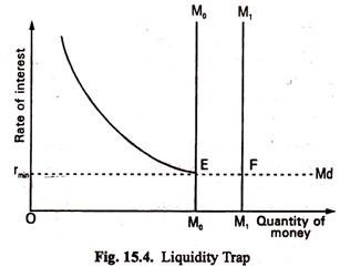
The implication is that monetary policy loses its effectiveness if there is a liquidity trap in the demand curve of money. Keynes argued that the only way to stimulate invest­ment in a depressed economy (which is experien­cing liquidity trap) is to use a positive fiscal policy. Such a policy works through an increase in government expenditure or reduction in taxes in order to increase aggregate effective demand.

The reason is simple. People feel that the rate of interest has fallen enough. It cannot fall further. Thus, if it rises in near future the price of bonds (purchased now) will fall. So purchase of bonds is risky. Money-holding is not that costly because the rate of interest is low.

Thus, people prefer to hold as much money as possible, with the expectation that the rate of interest will rise in future. As soon as it rises they will buy bonds. In such a situation any additional money supplied by the central bank will be absorbed by the people and this will prevent the rate of interest from falling further.

The Possibility of Zero Rate of Interest

Interest is treated as a price paid by borrowers to lenders and will depend on the supply for and demand of loanable money for various purposes. Generally, a large supply of capital relating to the demand means low rates of interest and a large demand relative to supply means high interest rates.

According to some writers, the rate of interest would fall to zero in a static economy where the demand for loanable funds is nil. In a static economy, there is no fresh investment, the demand for loanable funds is nil and so the rate of interest would be zero.

From the point of view of the demand for loans, zero rate of interest means that the marginal net product of capital is nil. This means that we cannot increase society’s total product further by employing more capital. We have reached a state in which our productivity is maximum. It means that all our wants have been satisfied. So the demand for capital will be zero.

But, it is not likely that the demand for loan-capital will be ever zero. But, in reality, we cannot think of a state of society in which people will have no wants, and no desires. So long as they remain, there will always be endless possibilities for employing capital. The rate of interest, therefore, cannot be zero.

There are certain dynamic forces like inventions and discoveries, growth of population, etc. which keep always up the demand price of loan-capital.

Similarly, from the supply side, a zero rate of interest means that people will go on lending without expecting any return in exchange. But the liquidity preference will not drop to zero for a number of reasons. As the rate of interest falls, more money will be absorbed by people to satisfy transactions demand for money.

Moreover, the zero interest rate means that the liquidity-preference also becomes zero; people lend money without any interest. But such a situation is most unlikely to appear in reality. There are always reasons why the liquidity-preference would never drop to zero.

As the holding of cash-money has the distinct advantages over the holding of other assets, people will always prefer cash money to other assets. It means that the liquidity- preference cannot drop down to zero, and from this it follows that the rate of interest will never fall to zero. All these set a limit much above zero to the practical decline in the rate of interest.

In the Keynesian theory it is also seen that the rate of interest cannot fall below a certain level where the demand for liquidity becomes infinitely elastic and that situation has already been described as the liquidity trap (Fig. 15.4), a term first used by D. Robertson.

David Ricardo, an English classical economist, first developed a theory in 1817 to explain the origin and nature of economic rent.

Ricardo used the economic and rent to analyse a particular question. In the Napoleonic wars (18.05-1815) there were large rise in corn and land prices.

Did the rise in land prices force up the price of corn, or did the high price of corn increase the demand for land and so push up land prices. Ricardo defined rent as, “that portion of the produce of the earth which is paid to the landlord for the use of the original and indestructible powers of the soil.” In his theory, rent is nothing but the producer’s surplus or differential gain, and it is found in land only.

Assumptions of the Theory

The Ricardian theory of rent is based on the following assumptions:

1. Rent of land arises due to the differences in the fertility or situation of the different plots of land. It arises owing to the original and indestructible powers of the soil.
2. Ricardo assumes the operation of the law of diminishing marginal returns in the case of cultivation of land. As the different plots of land differ in fertility, the produce from the inferior plots of land diminishes though the total cost of production in each plot of land is the same.
3. Ricardo looks at the supply of land from the standpoint of the society as a whole.
4. In the Ricardian theory it is assumed that land, being a gift of nature, has no supply price and no cost of production. So rent is not a part of cost, and being so it does not and cannot enter into cost and price. This means that from society’s point of view the entire return from land is a surplus earning.

Reasons for Existence of Rent

According to Ricardo rent arises for two main reasons:

1. Scarcity of land as a factor and
2. Differences in the fertility of the soil.

Scarcity Rent

Ricardo assumed that land had only one use—to grow corn. This meant that its supply was fixed, as shown in Figure 13.1. Hence the price of land was totally determined by the demand for land. In other words, all the price of a factor of production in perfectly inelastic supply is economic rent—it has no transfer earnings.

Thus, it was the high price of corn which caused an increase in the demand for land and a rise in its price, rather than the price of land pushing up the price of corn. However, this analysis depends on the assumption that land has only one use. In the real world a particular piece of land can be put to many different uses. This means its supply for any one use is elastic, so that it has transfer earnings.

Differential Rent

According to Ricardo, rent of land arises because the different plots of land have different degree of productive power; some lands are more fertile than others. So there are different grades of land. The difference between the produce of the superior lands and that of the inferior lands is rent—what is called differential rent. Let us illustrate the Ricardian concept of differential rent.

Differential Rent on account of differences in the fertility of soil:

Ricardo assumes that the different grades of lands are cultivated gradually in descending order—the first grade land being cultivated at first, then the second grade, after that the third grade and so on. With the increase in population and with the consequent increase in the demand for agricultural produce, inferior grades of lands are cultivated, creating a surplus or rent for the superior grades. This is illustrated in Table 13.1.

Table 13.1: Calculation of Differential Rent

Table 13.1 shows the position of 3 different plots of land of equal size. The total cost is the same for each plot of land. Let us assume that the order of cultivation reaches the third stage when all the three plots of land of different grades are cultivated and the market price has come to the level of Rs. 5 per kg of wheat.

The first grade land, being the most fertile, produces 40 kg, the second grade 70 kg and the third grade land, being less fertile, only 20 kg. So, the first grade land earns a surplus or rent of Rs. 100, the second grade a rent of Rs. 50 and the third one earns no surplus. The first two plots are called the intra-marginal and the third one is the marginal (or no-rent) land. This simple example shows how the differences in the fertility of the different plots of land create rent for the superior plots of lands.

The concept of differential rent arising due to differences in the fertility of different plots of land is illustrated in Fig. 13.2.

Here, AD, DG and GJ are three separate plots of land of the same size, but of difference in fertility. The total produce of AD is ABCD, that of DG is DEFG and that of GJ is GHIJ. The first and second plots of land generate a surplus shows by the shaded area, which represents the rent of the first two plots of land. Since the third plot GJ has no surplus it is marginal land or no-rent land. Grade 4 (below-marginal) land will not be cultivated, because rent is negative (Rs. 25 in this example).

Rent and Price

From the Ricardian theory we can show the relation between rent (of land) and price (of wheat). Since the market price of wheat is determined by costs of the marginal producer and since, for this marginal producer, rents are zero, Ricardo concluded that economic rent is not a determinant of market price. Rather, price of wheat is determined solely by the market demand for wheat and the availability of fertile land.

Deductions from the Theory

If rent depends on price and on the superiority of rent-producing land over marginal land, we can deduce the following:

1. Improved methods of farming:

Improved methods of cultivation may lead to a fall in rent (demand remaining unchanged). It is because increased output on the superior grades of land will make the cultivation of inferior grades of land unnecessary.

2. Population growth:

Population growth is likely to lead to a rise in rent, since the increased demand for land will bring poor quality land into cultivation, thus lowering the output of marginal land. Thus, if the price of food increases, the rent of existing land will increase.

3. Improved transport facilities:

Improved transport facilities are likely to lead to a fall in rent. It is because the output of less fertile land of foreign countries may be able to com­pete more closely with the home produce. So there will be no need to cultivate inferior home areas. As a result the output of the mar­ginal land rises and rent falls.

Thus, it is difficult to say whether or not rent increases with economic progress. How­ever, rent is likely to fall with economic pro­gress if population growth is unable to fully neutralise the effects of technological progress and improvement in transport facilities.

Criticisms of the Theory

Ricardian theory has been criticised on the following grounds:

1. Ricardo considers land as fixed in supply. Of course, land is fixed in an absolute sense. But land has alternative uses. So the supply of land to a particular use is not fixed (inelastic). For example, the supply of wheat land is not absolutely fixed at any given time.
2. Ricardo’s order of cultivation of lands is also not realistic. If the price of wheat falls the marginal land need not necessarily go out of cultivation first. Superior grades of land might cease to be cultivated if a fall in the price of its output causes such land being demanded for other purposes (e.g., for constructing houses).
3. The productivity of land does not depend entirely on fertility. It also depends on such factors as position, investment and effective use of capital.
4. Critics have pointed out that land does not possess any original and indestructible powers, as the fertility of land gradually dimi­nishes, unless fertilisers are applied regularly.
5. Ricardo’s assumption of no-rent land is unrealistic as, in reality; every plot of land earns some rent, although the amount may be small.
6. Ricardo restricted rent to land only, but modern economists have shown that rent arises in return to any factor of production, the supply of which is inelastic.
7. According to Ricardo, rent does not enter into price (cost) but from the point of view of an individual farm rent forms a part of cost and price.

Critical Evaluation of the Ricardian Theory

The Ricardian theory of rent has been the subject of many serious criticisms.

1. Ricardo’s concept of land is wrong. According to Ricardo, land possesses original and indestructible powers for which rent is paid. Critics, however, argue that land does not possess any original powers nor are its powers indestructible. For one thing, whatever fertility which land possesses now is mainly due to man’s effort-irrigation, manuring, drainage, etc. By using wrong agricultural practices, it is possible to destroy the properties of land.
2. Ricardo’s order of cultivation is faulty. Critics have found fault with Ricardo’s order of cultivation. According to Ricardo, the most fertile and most favorably situated land will be cultivated first. However, this may not always be the case. Even in a new country (about which Ricardo talks) the new settlers need not necessarily choose the best lands. They may not know which are the best lands.
3. The differential surplus concept of rent is defective. Ricardo assumes differential natural advantages of superior lands over inferior lands and bases his concept of rent on this difference. In the Ricardian analysis, if all lands possessed equal fertility, there would be no rent. Further in the Ricardian theory, the marginal land is a no-rent land. The supply of land is limited as compared to the demand for it and accordingly rent will exist because of the scarcity of land. All lands including the marginal land will secure rent.
4. The relation between rent and price is wrong. An important criticism leveled against Ricardian theory of rent concerns the relation between rent and price. According to Ricardo, price determines rent. The higher the price of corn, the higher will be the rent. The price of corn is determined by the cost of producing corn on the marginal land which is rent-free. Critics, however, disagree with Ricardo on this question. They argue that rent of land is a cost, and as such enters into the price of the product.
5. Rent is not peculiar to land. Modern economists argue that rent is not peculiar to land because differential surpluses similar to that of rent of land are widespread both in labour and capital payments. So long as a factor of production is inelastic (in relation to the demand for it) during a given period of time, a surplus income i.e., rent arises. There is no reason to argue that land alone can be fixed or inelastic in supply. Modern economists, therefore, have extended the concept of rent to refer to an income which any factor of production may secure over and above its minimum transfer cost.

Conclusion

In spite of the various short­comings of the Ricardian theory, it cannot be discarded—as Stonier and Hague remarked — “The concept of transfer earnings helps to bring the simple Ricardian theory of rent into closer relation with reality.”

The oldest and most significant theory of factor pricing is the marginal productivity theory. It is also known as Micro Theory of Factor Pricing.

It was propounded by the German economist T.H. Von Thunen. But later on many economists like Karl Mcnger, Walras, Wickstcad, Edgeworth and Clark etc. contributed for the development of this theory.

According to this theory, remuneration of cache factor of production tends to be equal to its marginal productivity.

Marginal productivity is the addition that the use of one extra unit of the factor makes to the total production. So long as the marginal cost of a factor is less than the marginal productivity, the entrepreneur will go on employing more and more units of the factors. He will stop giving further employment as soon as the marginal productivity of the factor is equal to the marginal cost of the factors.

Definitions

“The distribution of income of society is controlled by a natural law, if it worked without friction, would give to every agent of production the amount of wealth which that agent creates.” -J.B. Clark

“The marginal productivity theory contends that in equilibrium each productive agent will be rewarded in accordance with its marginal productivity.” -Mark Blaug

“The marginal productivity theory of income distribution states that in the long run under perfect competition, factors of production would tend to receive a real rate of return which was exactly equal to their marginal productivity.” -Liebhafasky

Assumptions of the Theory

The main assumptions of the theory are as under:

1. Perfect Competition

The marginal productivity theory rests upon the fundamental assumption of perfect competition. This is because it cannot take into account unequal bargaining power between the buyers and the sellers.

2. Homogeneous Factors

This theory assumes that units of a factor of production are homogeneous. This implies that different units of factor of production have the same efficiency. Thus, the productivity of all workers offering the particular type of labour is the same.

3. Rational Behaviour

The theory assumes that every producer desires to reap maximum profits. This is because the organizer is a rational person and he so combines the different factors of production in such a way that marginal productivity from a unit of money is the same in the case of every factor of production.

4. Perfect Substitutability

The theory is also based upon the assumption of perfect substitution not only between the different units of the same factor but also between the different units of various factors of production.

5. Perfect Mobility

The theory assumes that both labour and capital are perfectly mobile between industries and localities. In the absence of this assumption the factor rewards could never tend to be equal as between different regions or employments.

6. Interchangeability

It implies that all units of a factor are equally efficient and interchangeable. This is because different units of a factor of production are homogeneous, since they are of the same efficiency, they can be employed inter-changeable, and e.g., whether we employ the fourth man or the fifth man, his productivity shall be the same.

7. Perfect Adaptability

The theory takes for granted that various factors of production are perfectly adaptable as between different occupations.

8. Knowledge about Marginal Productivity

Both producers and owners of factors of production have means of knowing the value of factor’s marginal product.

9. Full Employment

It is assumed that various factors of production are fully employed with the exception of those who seek a wage above the value of their marginal product.

10. Law of Variable Proportions

The law of variable proportions is applicable in the economy.

11. The Amount of Factors of Production should be Capable of being Varied

It is assumed that the quantity of factors of production can be varied i.e. their units can either be increased or decreased. Then the remuneration of a factor becomes equal to its marginal productivity.

12. The Law of Diminishing Marginal Returns

It means that as units of a factor of production are increased the marginal productivity goes on diminishing.

13. Long-Run Analysis

Marginal productivity theory of distribution seeks to explain determination of a factor’s remuneration only in the long period.

Explanation of the Theory

The marginal productivity theory states that under perfect competition, price of each factor of production will be equal to its marginal productivity. The price of the factor is determined by the industry. The firm will employ that number of a given factor at which price is equal to its marginal productivity. Thus, for industry, it is a theory of factor pricing while for a firm it is a factor demand theory.

Analysis of Marginal Productivity Theory from the Point of View of an Industry

Under the conditions of perfect competition, price of each factor of production is determined by the equality of demand and supply. As the theory assumes that there exists full employment in the economy, therefore, supply of the factor is assumed to be constant. So, factor price is determined by its demand which itself is determined by the marginal productivity. Thus, under such conditions, it becomes essential to throw light on the demand curve or marginal productivity curve of an industry.

As the industry consists of a group of many firms, accordingly, its demand curve can be drawn with the demand curves of all the firms in the industry. Moreover, marginal revenue productivity of a factor constitutes its demand curve. It is only due to this reason that a firm’s demand or labour depends on its marginal revenue productivity. A firm will employ that number of labourers at which their marginal revenue productivity is equal to the prevailing wage rate.

Fig. 2 shows that at wage rate OP₁, the demand for labour is ON₁ and marginal revenue productivity curve is MRP₁. If wage rate falls to OP, firms will increase production by demanding more labour. In such a situation the price of the commodity will fall and marginal revenue productivity curve will also shift to MRP₂.

At OP wages, the demand for labour will increase to ON. DD₁ is the firm’s demand curve for labour. The summation of demand of all the firms shows demand curve of an industry. Since the number of firms is not constant under perfectly competitive market, it is not possible to estimate the summation of demand curves of all firms. However, one thing is certain that is the demand curve of industry also slopes downward from left to right. The point where demand for and supply of a factor are equal will determine the factor price for the industry. This theory assumes the supply of a factor to be fixed.

Thus factor price is determined by the demand for factor i.e. factor price will be equal to the marginal revenue productivity. It has been shown by Fig. 3. In the Fig. 3, number of labour has been taken on OX axis whereas wages and MRP have been taken on OY axis. DD₁ is the industry’s demand curve for labour. This is also the Marginal Revenue Productivity curve.

Factor Price (OW) = Marginal Revenue Productivity MRP.

Thus under perfect competition, factor price is determined by the industry and firm demands units of a factor at this price.

Analysis of Marginal Productivity Theory from the Point of View of Firm

Under perfect competition, number of firms is very large. No single firm can influence the market price of a factor of production. Every firm acts as a price taker and not a price maker. Therefore, it has to accept the prevailing price. No employer would like to pay more than what others are paying. In other words, a firm will employ that number of a factor at which its price is equal to the value of marginal productivity. Therefore, from the point of view of a firm, the theory indicates how many units of a factor it should demand.

It is due to this reason that it is also called Theory of Factor Demand. Other things remaining the same, as more and more labourers are employed by a firm, its marginal physical productivity goes or- diminishing. As price under perfect competition remains constant, so when marginal physical productivity of labour goes on diminishing, marginal revenue productivity will also go on diminishing. Therefore, in order to get the equilibrium position, a firm will employ labourers up to a point where their respective marginal revenue productivity is equal to their wage rate.

Table 2 indicates that wage rate of labour is Rs. 55 per labourers. Price of the product produced by the labourer is Rs. 5 per unit. Now, when a firm employs one labourer, his marginal physical productivity is 20 units. By multiplying the MPP with price of the product we get marginal revenue productivity. Here, it is Rs. 100 for the first labour. The marginal revenue productivity of second labourer is Rs. 85 and of third labourer it is Rs. 70.

The marginal revenue productivity of fourth labourer is Rs. 55 which is equal to wage rate. The firm will earn maximum profits if it employs up to the fourth labourer. If the firm employs fifth labourer, it will have to suffer losses of Rs. 15. Therefore, to get maximum profits, a firm will employ a factor upto a point where MRP is equal to price.

In Fig. 4 number of labourers has been measured on OX-axis and wage rate on Y-axis. MRP is marginal revenue productivity curve and WW is the wage rate prevailing in the market. Since, under perfect competition wage rate will remain constant that is why WW wage line is parallel to OX-axis.

MRP curve is sloping down-ward. It cuts WW at point E which is the equilibrium wage rate of Rs. 55. At point E, firm will demand only four labourers. Thus, from the above, we can conclude that a factor is demanded up to the limit where its marginal productivity is equal to prevailing price.

Under perfect competition, in long period in the equilibrium position, not only the marginal wages of a firm are equal to marginal revenue productivity, even the average wages of the firm are equal to average net revenue productivity as has been shown in Fig. 5. The fig. 5 shows that at point ‘E’ marginal wages of labour are equal to marginal revenue productivity and the firm employs OM number of workers. At this point, even the average net revenue productivity is equal to average wages. Thus firm earns only normal profit. If wage line shifts from NN to N[N] then the demand for labour increases from OM to OM₁.

Determination of Factor Pricing under Imperfect Competition

Marginal productivity theory applies to the condition of perfect competition. But in real life we face imperfect competition. Therefore, economists like Robinson, Chamberlin have analyzed factor pricing under imperfect competition. There are various firms under imperfect competition. But here we shall analyze only Monopsony. Under monopsony, there is perfect competition in product market. Consequently MRP is equal to VMP. There is imperfect competition in factor market.

It indicates that there is only one buyer of the factors. Therefore, monopsony refers to a situation of market where only a single firm provides employment to the factors. If the firm demands more factors, factor price will go up and vice-versa. However, the determination of factor price under monopsony can be explained with the help of Fig. 6.

In Fig. 6 number of labourers has been shown on X-axis and wages on Y-axis. MW is marginal wage curve and ARP is the average wage curve. MRP is the marginal revenue productivity curve and AW is the average revenue productivity curve.

In the fig. 6 a monopsony will employ that number of labourers at which their marginal wage is equal to MRP. In the fig. 6 firm is in equilibrium at point E. Here, firm will employ ON labourers and they will be paid wages equal to NF. In this way, ON labourers will get less wages than their MRP i.e. EN. Monopsony firm will have EF profit per labourer which arises due to exploitation of labourers. Total profit SFWW’ is due to exploitation of labour.

Prof. Knight’s theory of uncertainty bearing theory of Profit is an improvement and refinement theory of Profit over Hawley’s risk-bearing theory of Profit. Here, Profit according to Knight, is the reward of bearing non-insurable risks and uncertainties. It is a deviation arising from uncertainty.

Uncertainty prevails in the entire society and profits, positive or negative, in a way accrues to all factor services. In other words, there is profits element in all types of income. But the division of social income between Profit and contractual income depends on the supply of entrepreneurial ability.

Uncertainty bearing is the most important function in a dynamic state. It is the entrepreneur who either delegates this function among different personnel or assumes it himself. The expectation of Profit is, in a way, the supply price of entrepreneurial uncertainty-bearing. In a competitive economy where there is no risk, every entrepreneur will have a minimum supply price.

In short Knight’s theory implies that:

(i) Profit is reward for uncertainty-bearing.

(ii) The un-measurable risks are termed as uncertainty. These un-measurable risks are true hazards of business.

(iii) Pure Profit is, however, a temporal and unfixed reward. It is turned with uncertain­ty. Once the unforeseen circumstances become known, necessary adjustment would be possible. Then pure Profit disappears.

Its Criticisms:

Knight’s theory of Profit has been criticised on the following grounds:

a. This theory does not give clear notion of entrepreneurship therefore it has been called unrealistic:

In this theory there is no indication as to who are the real owners because owners are shareholders and policy decision-makers are salaried people.

b. Difficulty in the distribution of profit:

This theory does not solve the problem of allocation or distribution of profit among the controlling and ownership group, therefore, this theory keeps the problem of the determination of Profit unsolved.

c. This theory fails to expose the phenomenon of monopoly profit:

The theory does not suit well to expose the phenomenon of monopoly profit. When there is least uncertainty involved in a monopoly business.

d. Profit is not a residual income:

Knight has mentioned in his theory that Profit is a residual income but J. F. Weston has said that “the exercise of judgment of Profit may be sold on a fixed-price basis or on a variable price-basis.” This is how the expert manager sell their services to earn Profit.

e. This theory has not said anything on monopoly profit:

This theory does not throw any light on the monopoly profit. As we have studied that monopoly firms earn much larger profits than competitive firms and they are not due to the presence of uncertainty.

f. Above all, the uncertainty element cannot be qualified to improve profits.

In-spite of the weaknesses as mentioned above, this theory of Knight is regarded as the only satisfactory explanation of the nature of profit.

Meaning of Interest

In simple meaning interest is a payment made by a borrower to the lender for the money borrowed and is expressed as a rate percent per year.

It is usually expressed as an annual rate in terms of money and is calculated on the principal of the loan. It is the price paid for the use of other’s capital fund for a certain period of time.

In the real economic sense, however, interest implies the return to capital as a factor of production. But for all practical purposes, “interest is the price of capital.” Capital as a factor of production, in real terms, refers to the stock of capital goods (machinery, raw-materials, factory plant etc.).

In the money economy, however for all practical purposes capital refers to finance or money capital i.e., the monetary fund’s lent or borrowed for any purpose of expenditure from any source. In strict narrow sense, again, capital may refer to only funds borrowed for real investment in business by the business community from financial institutions.

Definition of Interest

In economics, Interest has been defined in a variety of ways. Commonly, Interest is regarded as the payment of the use of service of capital.

1. As Prof. Marshall has said – “The payment made by borrower for the use of a loan is called Interest.”
2. According to Prof. J. S. Mill – “Interest is the remuneration for mere abstinences.”
3. As Prof. Keynes has said – “Interest is the reward of parting with liquidity for a specified period.”
4. According to Seligman – “Interest is the return from the fund of capital.”
5. According to Carver – “Interest is the income which goes to the owner of capital.”
6. According to Richard – “Interest is primarily a reward for waiting.”
7. As per the opinion of Prof. Wicksell – “Interest may be defined as a payment made by the borrower of capital by virtue of its productivity as a reward for his capitalist’s abstinence.”

But the modern economist in order to avoid the divergent and controversial views about Interest, have explained it in terms of productivity, saving, liquidity and money. In other words, Interest is the reward for the yield of capital, of saving, for the foregoing of liquidity and the supply of money. Thus, they have explained it in terms of the demand and supply of money

Why Interest is Paid or Charged

There are two views regarding Interest paid or is charged:

(i) From Debtor’s point of view,

(ii) From Creditor’s point of view.

From Debtor’s Point of View

Debtor’s pay interest on capital because he is aware that capital has productivity and if it can be used in production there can be increase in income. Therefore, out of the earned income, a part of the income is paid to the creditor or a lender from whom money has been taken as loan is known as Interest.

Following are the important reasons for giving Interest:

Use of Capital:

Whatever amount is paid to the owner of the capital for the use of the capital is known as Interest. Here, the capital is used in further production and whatever he earns, he pays a part of his earnings to the owner of the capital or the lender of the money.

Reward for Risk:

Loan giving is a risk which lender takes at the time of giving loan or advancing money. Lender exposes himself to risk when he lends money and sometimes the loan become bad-debts. Therefore, it has been said that Interest is the reward for risk taking.

Interest is Reward for Inconvenience:

When a lender gives loan of money he forgets its use for the duration of the loan, if he needs this amount for his personal use, he will have to undergo the inconvenience of arranging it from some other source. Thus, he feels inconvenience.

Expenses in Relation to Management of Business:

For organising and running the business, businessman needs money. Money taken as loan for running and managing business, keeping accounts, maintaining standard of business etc. one has to arrange money and for that has to pay interest over the money.

From Creditor’s Point of View

Creditors or lender of money demands Interest because he has taken pains in saving money, has suffered inconveniences in postponing his needs and has taken risk of bad debts. If he will not get Interest or some advantage of Interest he may loose interest in saving money or he may not be ready to bear inconveniences. Then, the formation of capital in the market will stop. Therefore, it can be said that the debtor’s give Interest to creditors as capital has productivity and creditors demand interest as the lender of money has taken risk and has faced inconveniences, so he must get some reward for the pains of inconvenience and risk.

Types of Interest

There are two types or kinds of Interest:

(a) Net Interest,

(b) Gross Interest.

(a) Net Interest:

The payment made exclusively for the use of capital is regarded as net Interest or pure Interest. According to Prof. Chapman—“Net Interest is the payment for the loan of capital when no risk, no inconveniences apart from that involved in saving and no work is entailed on the lender.”

According to Prof. Marshall, “Net Interest is the earnings of capital simply or the reward of waiting simply.”

Thus, Net Interest = Gross Interest – (payment for risk + payment for inconvenience + cost of administering credit)

i.e., Net Interest = Net Payment for the use of capital.

(b) Gross Interest

Gross Interest according to Briggs and Jordan has said—“Gross Interest is the payment made by the borrowers to the lenders is called Gross Interest or Composite Interest.”

It includes payments for the loan of capital payment to cover risks for loss which may be:

(i) A personal risks or

(ii) Business risks, payment for inconveniences of the investment and payment for the work and worry involved in watching—investments, calling them in and investing.

According to Prof. Marshall:

Gross Interest is that “Interest of which we speak when we say that interest is the earning of capital simply or the reward of waiting simply, is net Interest but what commonly passes by the name of interest, includes other elements besides this and may be called gross interest.”

By seeing the above definitions when we add elements of payment for risk, payment for inconvenience and the cost of administering credit to the net Interest, it becomes gross interest.

Thus, Gross Interest = Net Interest + payment of risk + payment for inconvenience + cost of administrating credit

Elements of Gross Interest

As we have seen earlier that the actual amount paid by the borrower to the capitalist as the price of capital fund borrowed is called gross interest.

Gross interest includes, besides net interest, the following elements:

1. Payment or Compensation for Risk

The lender has always to bear the risk—the risk that the loan may not be repaid. Besides this, borrower, takes the loan at the time when his requirement is urgent but when he returns it, it is quite possible that the time may not be suitable from lender’s point of view. To cover this risk, the lender charges more, in addition to the net interest. Thus, when loans are made without adequate security, they involve a high elements of risk, so a high rate of Interest is charged.

2. Compensation for Inconvenience

When somebody lends the money, he has to bear inconveniences till the period when he gets back the sum, i.e., a lender lends only by saving that is by restricting consumption out of his income which obviously involved some inconveniences which is to be compensated.

A similar inconvenience is that the lender may be able to get his money back as and when he may need it for his own use. Hence, a payment to compensate this sort of inconvenience may be charged by the lender. Thus, the greater the degree of inconvenience caused to the lender, higher will be the rate of Interest charged.

3. Cost of Administering the Credit or Payment for Management Services

A lender of capital funds has to spend money and energy in the management of credit.

For example:

In the lending business, certain legal formalities have to be fulfilled, say fees for obtaining money-lender’s licence, stamp duties etc. Proper accounts must be maintained. He has to maintain a staff as well. For all these sorts of management services, reward has to be paid by the borrower to the lender. Therefore, gross interest also includes payment for management expenses.

4. Compensation for the Changing Value of Money

Under this when prices are rising, the purchasing power of money declines over a period of time and the creditor loses. To avoid such loss and high rate of Interest may be demanded by the lender.

Therefore,

Gross Interest = Net Interest + Payment for risk + Payment for management services + Compensation for the changing value of money.

In economic equilibrium, the demand and supply for capital determines the net rate of interest. But in practice, gross interest rate is charged. Gross interest rates are different in different cases at different places and different times and for different individuals.

Factors Influencing the Rate of Interest

Interest rates vary from person to person and from place to place.

There are many factors which causes variations in Interest rates which Eire as such:

1. Different Types of Borrowers

There are different types of borrowers in the market. They offer different types of securities. Their borrowing motives and urgency are different. Thus, the risk elements differ in different cases, which have to be compensated for.

2. Due to Differences in Gross Interest

Variations in the rate of Interest are due to differences in gross interest such as risk and inconveniences involved, cost of keeping records and accounts and collection of loans etc. The greater the risk and inconvenience and the cost of management of loans, the higher will be the rate of Interest and vice-versa.

3. The Money Market is not Homogeneous

There are different types of lenders and institutions, specialising in different types of loans and the loan-able funds are not freely mobile between them. The ideals of these institutions are also different. Again, there are moneylenders and indigenous bankers in the unorganised sector of the money market who follow their distinct lending policies and charge different interest rates.

4. Duration of Loan or Period of Loan

Rate of Interest also depends upon the duration or period of loan. Larger term loans carry higher rate of Interest than short-term loans. In a long-term loan, the money gets locked up for a longer duration. Naturally, the lender wants to be compensated by a higher rate of Interest.

5. Nature of Security

Interest rate varies with the type of security. Loans against the security of gold carry less interest rates than loans against the security of gold carry less interest rate than loans against the security of immovable property like land or house. The more liquid are the assets the lower is the interest rate and vice-versa.

6. Goodwill or Credit of the Borrower

Interest rate also depends upon the credit or goodwill of the borrower. Persons of better goodwill and known integrity and credibility can get loans on easy terms.

7. Amount of Loan

The greater the amount of loan, the lower is the rate of Interest and vice-versa.

8. Interest Policy of the Monetary Authorities

Monetary policy of the authorities may also lead to differences in Interest rates, e.g., the Reserve Bank of India has adopted differential interest rates policy for the deployment of credit to the priority sectors.

9. Difference Due to Distance

Distance between the lender and the borrower also causes differences between Interest rates. People are willing to lend at a lower rate of Interest nearer home than at a long distance.

10. Market Imperfections

Differences in Interest rates are also due to market imperfections that may be found in a loan market. Money-lenders indigenous banks, mutual funds, commercial banks etc. follow different lending policies and charges various Interest rates.

11. Differences in Productivity

Productivity of capital differs from work to work or from venture to venture. People are willing to borrow at a higher rate of Interest for productive purposes or productive ventures and vice-versa.

Grounds in which Payment of Interest is Justified

The payment of Interest is justified on various grounds.

The following are the reasons for payment of Interest:

1. The Productivity of Capital

Interest is paid by the borrower to the lender, because borrowed money capital is productively used.

2. Compensation for Parting with Liquidity

As Keynes has said that interest is the reward for parting with liquidity when a lender lends money he undergoes a sacrifice of present time consumption is parting with its purchasing power to the borrower. This is to be compensated by the borrower to the lender by paying a rate of Interest as agreed upon.

3. To Induce Savings

Lending of money mostly comes out of savings. Savers are induced to save more by restricting consumption, when high rates of Interest are paid. When investment demand is in excess of savings, Interest rates will go up.

4. To Mobilise Loan-Able Funds

Banks and other financial institutions offer Interest rates to mobilise loanable funds from the household sector to the money and capital markets. People may opt for financial investment of their savings when attractive returns are offered by the financial institutions. Financial institutions serve as intermediaries and pass on these funds so mobilised to the firm sector for real investment.

Similarly, the demand for Interest on the lender’s side is also justifiable for the reason for abstinence or sacrifice of immediate consumption undergone by them in parting with liquidity. They also claim a share in the income generated by capital in its productive use in terms of Interest rate. They also face the risk of losing money when the loan is not repaid by the borrower. To compensate for all these risk elements, they reasonably demand some Interest.

The Classical Theory of Interest

The classical theory of interest also known as the demand and supply theory was propounded by the economists like Marshall and Fisher.

Later on, Pigou, Cassel, Knight and Taussig worked to modify the theory.

According to this theory rate of interest is determined by the intersection of demand and supply of savings. It is called the real theory of interest in the sense that it explains the determination of interest by analyzing the real factors like savings and investment. Therefore, classical economists maintained that interest is a price paid for the supply of savings.

Demand for Savings

Demand for savings comes from those who want to invest in business activities. Demand for investment is derived demand. Any factor of production is demanded for its productivity. The demand for the factor is high when there are higher expectations from it.Since, all the factors are not equally productive, so, capital demand will be high for more productive uses first and then gradually with the increase in its supply, will shift to less productive uses.

Therefore, classical economists maintained that with the aid of capital facilities we turn out more goods per man-hour than when we produce with bare hands or with scant tools. Moreover, marginal productivity of the business goes on decreasing with more and more doses of investment of savings in his business venture. It is due to the operation of the law of diminishing returns.

Now a very important question arises is that how much capital a person will demand because when a person borrows money he has to pay interest on it. The answer according to this theory is that demand for capital can be raised to a point where marginal productivity of capital becomes equal to the interest paid on it. Thus, if marginal productivity of capital is more than the interest paid, then it is beneficial to borrow money and vice-versa. Equilibrium will prevail at a point where marginal productivity of capital equals the rate of interest. This shows that there exists inverse relationship between demand for capital and the interest rate.

This fact can be made clear with the help of the following table 1 and diagram 1:

Table 1 shows that rate of interest and investment are inversely related to each other. As the rate of interest increases, the level of investment declines and vice-versa. As in the table, initially, the rate of interest is 10%, investment is Rs. 500 crores. When the rate of interest decreases to 8%, the level of investment increases to Rs. 700 crores from Rs. 500 crores. Further, as the rate of interest again falls to 5%, the level of investment increases to Rs. 1000 crores.

The Fig. 1 depicts that there exists inverse relationship between the investment and the rate of interest. Initially, the rate of interest is 10%, the level of investment is Rs. 500 crores. Now the rate of interest falls to 5%. With this decrease in the interest rate, level of investment increases to Rs. 1000 crores. It indicates that more capital is demanded at a low interest rate and vice versa.

Supply of Savings

Supply of capital is the result of savings. It comes from those who have the excess of income over consumption. Thus, savings is the main source of capital which depends on the capacity to save, willingness to save, level of income and rate of interest etc. Capacity to save depends on the size of national income, size of personal income, size of family, price level and purchasing power of money etc. Willingness to save depends on the family affection, further expectations etc.

To a large extent, willingness to save is affected by the rate of interest. On a higher rate of interest people save more to earn the benefits of high rate of interest. On the other hand, at the low rate of interest, people save less. Thus, we may say that there is a direct relationship between the supply of savings and the rate of interest. The following table and diagram justifies this fact in a more vivid way.

It is clear from the table 2 that rate of interest and savings have a positive relationship. As the rate of interest increases, savings will also increase. On the other hand, a fall in rate of interest leads to a decrease in savings. When the rate of interest is 10%, the savings are of Rs. 1000 crores.

In the successive periods, as rate of interest falls from 10% to 5%, the total savings also decline. Suppose as the rate of interest falls to 5%, savings also decrease to Rs. 400 crores.

In Fig. 2 savings have been represented on X-axis and interest rate on Y-axis. SS is the supply curve which moves upward from left to right. It shows that supply of savings is interest elastic. Higher the interest rate, more will be saved and vice-versa. With 5% rate of interest money savings are Rs. 400 crores. As the interest rate increases to 10% people are persuaded to save more and the money savings rise to Rs. 1000 crores. This signifies that there is a direct relationship between savings and the rate of interest.

Equilibrium Rate of Interest

According to classical theory, equilibrium interest rate is restored at a point where demand for and supply of capital are equal i.e.

The table 3 reveals that equilibrium rate of interest will be determined at a point where demand for and supply of capital are equal. As is clear from the table that equilibrium interest rate 8% is determined because at this level demand for and the supply of capital are equal i.e. Rs. 700 crores.

Now, if the rate of interest increases to 10%, investment is Rs. 500 crores and savings are of Rs. 1000 crores i.e. savings exceed the investment. On the other hand, if the rate of interest falls to 5% investment is Rs. 1000 crores and savings are Rs. 400 crores.

This fact is clearer from the diagram below:

In Fig. 3, rate of interest is determined by the intersection of demand and supply curves. Equilibrium is restored at point E which determines rate of interest as 8% and demand and supply of capital as Rs. 700 crores. Now, if the rate of interest increases to 10% supply of savings exceeds the demand for capital i.e. supply is more than demand. This will lead to a fall in interest rate to the level of 8%.

On the other hand, when the interest rate falls to 6%, demand for savings exceeds the supply of savings which will push up the rate of interest to restore an equilibrium rate i.e. 8%. Therefore, rate of interest is in equilibrium only at a point where the demand for capital equals the supply of capital.

Criticism

The classical theory of rate of interest has been criticized on the basis of the following shortcomings as discussed below:

1. Indeterminate Theory:

Keynes has maintained that the classical theory is indeterminate in the sense that it fails to determine the interest rate. In this theory, interest is determined by the equality of demand and supply. But the position of savings varies with the income level. Thus, unless we know the income, interest rate cannot be determined.

2. Fixed Level of Income:

Classical theory assumes that the level of income remains constant. But in actual practice income changes with a small change in investment. Thus, it is not correct to assume a fixed level of income.

3. Long Run:

Classical theory determines the interest rate through the interaction of demand and supply of capital in the long run. Keynes pointed out that in the long run we all are dead. Therefore, there was an urgent need of a theory which determines rate of interest in the short-run.

4. Full Employment:

This theory assumes that there is full employment of resources in the economy. But, in reality, unemployment or less than full employment is a general situation. Full employment is only an abnormal case… Thus, this theory does not apply to the present world.

5. Savings and Investment:

Classical economists assume that savings and investment are interring dependent. But actually investment changes, income also changes which leads to a change in savings. Thus, both are interdependent on each other.

6. Ignores Monetary Factors:

Classical theory takes into consideration only the real factors for determining the rate of interest and ignores the monetary factors.

Introduction

The Marginal Productivity Theory of Wages is a fundamental concept in economic theory that explains how wages are determined in a competitive labor market. This theory, primarily developed by John Bates Clark and further refined by other neoclassical economists, asserts that wages are determined by the marginal productivity of labor. In other words, each worker is paid according to the additional output they contribute to the firm.

This theory is widely accepted for its logical appeal and its ability to explain wage determination in a market economy. However, it has also faced extensive criticism due to its simplistic assumptions and inability to account for real-world complexities such as market imperfections, labor unions, and employer-employee power dynamics. This essay provides a detailed and fact-based critical discussion of the marginal productivity theory of wages, examining both its strengths and limitations.

Understanding the Marginal Productivity Theory of Wages

The marginal productivity theory of wages states that in a perfectly competitive labor market, an employer will continue to hire workers until the marginal revenue product of labor (MRPL) equals the wage rate. The marginal revenue product of labor is the additional revenue generated by employing one more worker. This means that:

$$Wage=MRPL=M{P}_L\times P$$

Where:

• MP_L = Marginal Product of Labor (additional output from hiring one more worker)
• P = Price of the product in the market

According to this theory, firms are profit maximizers and will not pay workers more than what they contribute to production. If a worker’s marginal product exceeds their wage, the firm will benefit from hiring more workers. Conversely, if the wage exceeds the worker’s contribution, the firm will reduce employment.

Assumptions of the Marginal Productivity Theory of Wages

The theory is based on several critical assumptions, which make it mathematically elegant but limit its practical application:

• Perfect Competition: Both the labor market and the product market are assumed to be perfectly competitive. This means no single firm or worker has the power to influence wages.
• Homogeneous Labor: All workers are assumed to have the same skill set, and there are no differences in productivity between individuals.
• Diminishing Marginal Productivity: The contribution of each additional worker to production decreases as more workers are hired, assuming capital and technology remain constant.
• Full Employment: The theory assumes that all individuals who are willing and able to work at the equilibrium wage will find employment.
• Labor is a Variable Factor: Firms can freely adjust the number of workers they employ according to wage changes.

These assumptions create a theoretical ideal, but they fail to account for real-world labor market conditions, which are far more complex and often deviate from these idealized assumptions.

Strengths of the Marginal Productivity Theory of Wages

Despite its limitations, the marginal productivity theory of wages has several strengths that contribute to its acceptance in economic thought:

• Logical and Mathematically Sound: The theory provides a clear mathematical framework for understanding how wages are determined.
• Efficiency in Resource Allocation: It explains how resources, including labor, are allocated efficiently in a competitive market. If firms pay workers according to their marginal productivity, labor is allocated to its most productive use.
• Foundation for Wage Determination: The theory provides a foundation for understanding why wages differ across industries and occupations based on differences in marginal productivity.
• Explains Wage Differences in Competitive Markets: Higher wages in some professions can be attributed to higher marginal revenue productivity, such as in technology or finance, where workers contribute significantly to revenue.

Criticisms of the Marginal Productivity Theory of Wages

Despite its strengths, the theory has been widely criticized for failing to explain wage determination accurately in the real world. Some of the major criticisms include:

1. Unrealistic Assumptions

The theory assumes perfect competition, which is rarely observed in real labor markets. In reality, labor markets are characterized by monopsony power, trade unions, minimum wage laws, and imperfect information. Employers often have more bargaining power than workers, which leads to wage suppression.

2. Neglect of Institutional Factors

The theory ignores the role of government policies, labor unions, minimum wages, and collective bargaining, all of which play a significant role in wage determination. In many countries, wage floors and legal protections prevent wages from falling to the level determined solely by marginal productivity.

3. Wage Rigidity and Market Imperfections

In real-world labor markets, wages are often sticky and do not adjust immediately to changes in marginal productivity. Factors such as long-term contracts, social norms, and psychological considerations lead to wage rigidity, which the theory does not explain.

4. Inequality and Disparities

The marginal productivity theory does not account for historical inequalities, discrimination, and barriers to entry in certain professions. If wages were determined solely by marginal productivity, then discrimination based on gender, race, or class should not exist. However, empirical evidence shows that wage disparities persist despite similar productivity levels.

5. Role of Human Capital and Skill Differences

The theory assumes that labor is homogeneous, but in reality, workers have different education levels, experience, and skills. The concept of human capital, introduced by economists such as Gary Becker, suggests that differences in wages are partly explained by differences in investment in education and training, which the marginal productivity theory does not fully capture.

6. Difficulty in Measuring Marginal Productivity

Determining the exact marginal productivity of a worker is extremely difficult, especially in service-based and knowledge-intensive industries. For example, in healthcare or education, it is challenging to quantify the precise contribution of an individual worker to output.

7. Automation and Technological Unemployment

With the rise of automation and artificial intelligence, the marginal productivity of labor is being disrupted. In some cases, machines and algorithms replace human labor, reducing the marginal productivity of workers in certain industries. The theory does not adequately address how technological advancements alter wage structures.

Empirical Evidence and Real-World Application

Empirical studies show that wages are influenced by a variety of factors beyond marginal productivity. For instance:

• In developed economies, wage differences are significantly affected by labor market institutions, bargaining power, and government policies.
• In developing countries, informal employment and lack of strong labor protections lead to wages being determined by factors such as social networks, discrimination, and employer dominance, rather than marginal productivity alone.
• Research on gender wage gaps shows that even when productivity differences are accounted for, women often earn lower wages than men due to structural and societal factors.

Conclusion

The Marginal Productivity Theory of Wages provides an important theoretical foundation for understanding wage determination in a competitive labor market. It explains how firms make hiring decisions based on the additional output contributed by workers. However, its rigid assumptions and failure to account for real-world complexities make it an imperfect model for actual labor markets.

While the theory offers valuable insights into the relationship between productivity and wages, it oversimplifies labor market dynamics by ignoring institutional, social, and economic realities. In modern economies, factors such as minimum wage laws, trade unions, wage bargaining, discrimination, and technological advancements significantly impact wages, making it necessary to consider alternative theories alongside marginal productivity theory.

Thus, while the marginal productivity theory remains a cornerstone of neoclassical economic thought, it must be supplemented with real-world considerations to develop a more accurate and comprehensive understanding of wage determination.